Control Theory

• dynamical systems
  • one goal: modelling, taking in data, and predicting what happens; i.e. revealing the workings of the black box
  • alternative: you want to control this system, by controlling the inputs
• active control
  • open-loop: without looking at the output, have some set of inputs that produces desirable outputs
  • closed-loop (feedback control): through the use of sensors (that can measure the output), pick inputs that are functions of the output.
• example: inverted pendulum
  • it turns out that if the base oscillates sinusoidally, then you can actually make it stable. this is an example of open-loop. you don’t care about the output, all you do is have some preplanned input sequence to stabilize the system
  • a human would not do that, but basically balance the pendulum. this is responding to the data (or state of the system), so it’s closed-loop.
  • here, the state of the system can be captured by the angle, vector of acceleration (first and second moments?)
• why feedback?
  • Uncertainty (mis-specification of the model)
    • with open-loop, you’re assuming your model is exactly right, so your pre-planned sequence might be ideal. but if your model is wrong, then you can’t do anything.
    • so this is related to robustness (sort of). by having it be adaptive, then you can set it up to handle mis-specification, and be able to handle different scenarios (I assume even changing dynamics).
  • Instability
    • in the inverted pendulum example, with open-loop, you’re not changing the dynamics of the system itself (unstable eigenvalue)
    • however, when you have feedback, you can actually change the system dynamics
  • Disturbances (gust of wind, exogenous forces)
    • open-loop, you can’t handle extreme events (since you’re not measuring output)
    • closed-loop, you can correct
  • Efficiency
    • with elegant feedback control, it’s just much more efficient (besides the fact that you have to track the output)

Consider a state-space variable \(X\). Then, assume a linear dynamical system (ODE): \(\dot{x} = Ax\). Then its solutions are \(x(t) = e^{At} x(0)\), which means that if \(A\) has eigenvalues with positive real part, then the system is unstable (conversely, if all real parts of the eigenvalues are negative, then it’ll stabilize).

In Control, the dynamic is then \(\dot{x} = Ax + Bu\), where \(u\) is some actuator (that can basically change the input). Let \(u = -Kx\) is our control law. This then gives \(\dot{x} = (A - BK)x\), which means you’ve actually changes the dynamics of the system(!). Thus, you are able to turn an unstable system to a stable one.

LQR

episode

Linear Quadratic Regularizer: how do you pick \(K\) (the control law), or the negative eigenvalues? Basically what you can do is set up a cost function for your \(x\) (control how much you want these things to change) and \(u\) (control how much energy you’re willing to expend), and have weights \(Q,R\) you pick for what you care about. Then, it turns out that there is a closed form solution for the \(K\) that minimizes the cost function below:

\[ \begin{align*} \int_{0}^{\infty} \left( x^\top Q x + u^\top R u \right) dt. \end{align*} \]

Recall that \(u = -Kx\), and so the system dynamics is still \(\dot{x} = (A - BK)x\), and so you can simply parameterize everything with respect to time \(t\).

Kalman Filter

In class, we motivate Kalman filters as gaussian versions of a hidden markov model (HMM). From a control perspective, it is essentially an optimal procedure to recover the state space (\(x\)) from the output \(y\). The LQR above requires you to know the whole state space (I think?), so the KF gives \(\hat{x}\), and comes before the LQR step.

Loop Transfer

Shifting gears, let’s look at transfer functions.11 Basically you can think of this as our typical functional approach to ML, but taking inputs in the fourier domain instead (so \(\omega\)’s). Define our loop transfer function as \(L = PK\).

Figure 1: Loop Transfer Diagram

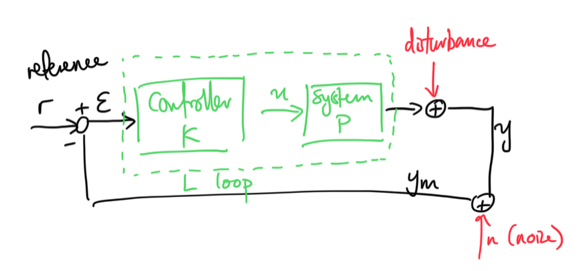
Here we are thinking of some reference state we want to achieve (say some speed in cruise control). \(K\) and \(P\) are transfer functions, and the disturbance might also be a transfer function \(P_d\) applied to \(d\) (recall that disturbance is some unmodelled aspect, versus just noise (\(n\) here)).

The master equation is given by \[ \begin{align*} y = P_d d + PK(\overbrace{r - y - n}^{\epsilon}). \end{align*} \] Solving for \(y\) gives \[ \begin{align*} y = (I + PK)^{-1} PKr + (I + PK)^{-1} P_d d + (I + PK)^{-1} PK n. \end{align*} \] Set \(S = (I+L)^{-1}\) (sensitivity) and \(T = (I+L)^{-1}L\) (complementary sensitivity), and note that \(S + T = I\). Then, in terms of the error, \[ \begin{align*} \epsilon = r - y_m = Sr - S P_d d + Tn \end{align*} \]

The only thing we can pick is \(K\), so we’re going to want to pick our law such that it has:

• good performance: we have some reference \(r\), so we want \(y \approx r\).
• reject disturbances: second term (transfer function) should be small
• attenuate noise: third term (at high frequencies, which is probably noise, we make this term small)

So actually what we get is that for small frequencies we want small \(\log |S|\), while for high frequencies, we want small \(\log |T|\) (at least for common physical systems like cruise control).

Robustness

(hand-wavy section mainly for intuition, following episode)

The above system (with LQR and KF) is optimal control, and was the mainstay of Control for a long time. This has optimality properties under various model assumptions. The question is, how robust is this to uncertainty, which we mentioned above – the fact that our models cannot perfectly capture the reality of the system (model mis-specification in statistics); plus a new idea, time-delay, which is just the reality that there’s going to be delay between getting the output and being able to actuate the systems/inputs.

In Control, the way to deal with robustness is actually fairly simple. What it boils down to is ensuring that your system never reaches a particular point (akin to the Nyquist stability condition, but essentially stay away from \(1+0i\)). I think the way it works is that you characterize the open-loop dynamics, which I assume means without feedback. Then, there are certain configurations such that when you close the loop, by adding your LQR, then you’re basically going to screwed.

The idea of robustness is that basically we can perfectly characterize the dynamics of the system, but uncertainty means we actually want a band around that modelled dynamics, an amount of slack that we are able to handle without the system becoming destabilized.22 The key thing for Control is all about this notion of stability, which is very unlike robustness in statistics. Since they’re dealing with dynamics, that’s really the end-game, which makes sense.

Recall sensitivity \(S = (I + L)^{-1}\), which is essentially the denominator term when you look at the closed loop solution \(y = \frac{PK}{1 + PK} r\). Then, the minimum distance from \(-1+0i\) relates to \(S\), so upper-bounding the maximum \(S\) is the same as controlling how close the system is to instability.

It turns out that time-delay (plus this notion of RHP zeros of \(P\)), both of which are different forms of uncertainty, gives fundamental bounds on the minimum distance (or maximum sensitivity) allowed in the system. That is, if your system has time-delay, then there is just some prescribed maximum \(S\) that your system can handle. This makes sense intuitively since if there is a time-delay then you basically can’t react fast enough to recover the system.33 Not sure if this intuition is the same as that of the stability condition.

Model Predictive Control

episode

How to handle non-linear? Suppose you have some reference desirable state. Then, at each time step, what you’re going to is basically project forward by some finite time horizon (\(k\) steps, say), and optimize your control law (the parameters) to minimize the difference between your reference state and the final state (in some metric).

Then, the wierd thing is that you basically just take the first step, and redo it all again. I guess the point here is that because things are non-linear, and your prediction model might not be great – also, since everything is feedback-based, it doesn’t really make sense to just project the next few steps and just go with what you predict (that also means you’re not adapting to differences between your projection and the truth).44 Of course this is just scratching the surface – I can imagine instances whereby if your predictions are close to the truth, then you might just go with your predicted steps, and not have to rerun the simulations.

This a general framework that’s very different from the LQR, not only in that it is non-linear, but also because it’s an online procedure, unlike the rest. LQR is an offline procedure: you model the system, I guess you have to work out what the parameters55 I guess this is where adaptive control comes into play, learning the parameters in the process (which dad says involves gradient descent, unsurprisingly)., but once you do, then the law is just a straightforward function.

MPC, on the other hand, is constantly evolving (i.e. online).

Takeaways

• Control is not afraid of model misspecification (or disturbances). The point of feedback is that you’re able to handle such things.
• Time-delay has a huge impact on robustness.
• The primary goal in Control is stability; then, performance. Or, I guess the point of robust control is that you can have both.