#gradient_descent
Exponential Learning Rates
via blog and (Li and Arora 2019Li, Zhiyuan, and Sanjeev Arora. 2019. “An Exponential Learning Rate Schedule for Deep Learning.” arXiv.org, October. http://arxiv.org/abs/1910.07454v3.)
Two key properties of SOTA nets: normalization of parameters within layers (Batch Norm); and weight decay (i.e \(l_2\) regularizer). For some reason I never thought of BN as falling in the category of normalizations, ala [[effectiveness-of-normalized-quantities]].
It has been noted that BN + WD can be viewed as increasing the learning rate (LR). What they show is the following:
The proof holds for any loss function satisfying scale invariance: \[ \begin{align*} L(c \cdot \theta) = L(\theta) \end{align*} \] Here’s an important Lemma:
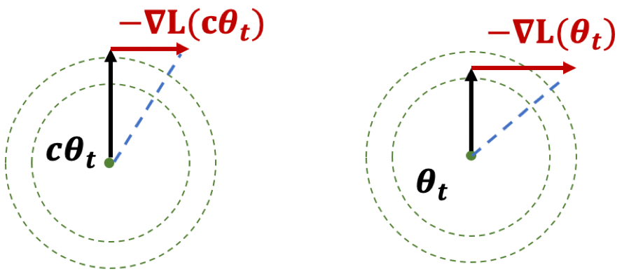 Figure 1: Illustration of Lemma
The first result, if you think of it geometrically (Fig. 1), ensures that \(|\theta|\) is increasing. The second result shows that while the loss is scale-invariant, the gradients have a sort of corrective factor such that larger parameters have smaller gradients.
Thoughts
The paper itself is more interested in learning rates. What I think is interesting here is the preoccupation with scale-invariance. There seems to be something self-correcting about it that makes it ideal for neural network training. Also, I wonder if there is any way to use the above scale-invariance facts in our proofs.
They also deal with learning rates, except that the rates themselves are uniform across all parameters, make it much easier to analyze—unlike Adam where you have adaptivity.
The Unreasonable Effectiveness of Adam
Intuition about Adam / History
We talk about gradient descent (GD), which is a first-order approximation (via Taylor expansion) of minimizing some loss, and Newton’s method (NM) is the second-order version. The key difference is in the step-size, which, in the second-order case, is actually the inverse Hessian (think curvature).
Nesterov comes along, wonders if the GD is optimal. Turns out that if you make use of past gradients via momentum, then you can get better convergence (for convex problems). This is basically like memory.
What remains is still the step-size, which needs to pre-determined. Wouldn’t it be nice to have an adaptive step-size? That’s where AdaGrad enters the picture, and basically uses the inverse of the mean of the square of the past gradients as a proxy for step-size. The problem is that it treats the first gradient equally to the most recent one, which seems unfair. RMSProp makes the adjustment by having it be exponentially weighted, so that more recent gradients are preferentially weighted.
Adam (Kingma and Ba 2015Kingma, Diederik P, and Jimmy Lei Ba. 2015. “Adam: A method for stochastic optimization.” In 3rd International Conference on Learning Representations, Iclr 2015 - Conference Track Proceedings. University of Toronto, Toronto, Canada.) is basically a combination of these two ideas: momentum and adaptive step-size, plus a bias correction term.1 I didn’t think much of the bias correction, but supposedly it’s a pretty big deal in practice. One of its key properties is that it is scale-invariant, meaning that if you multiply all the gradients by some constant, it won’t change the gradient/movement.
One interpretation proffered in the paper is that it’s like a signal-to-noise ratio: you have the first moment against the raw (uncentered) second moment. Essentially, the direction of movement is a normalized average of past gradients, in such a way that the more variability in your gradient estimates, the more uncertain the algorithm is, and so the smaller the step size.
In any case, this damn thing works amazingly well in practice. The thing is that we just don’t really understand too much about why it does so well. You have a convergence result in the original paper, but I’m no longer that interested in convergence results. I want to know about #implicit_regularization.
Adam + Ratio
Let’s consider a simple test-bed to hopefully elicit some insight. In the context of the [[project-penalty]]: we want to understand why Adam + our penalty is able to recover the matrix. In our paper, we analyze the gradient of the ratio penalty, and give some heuristics for why it might be better than just the nuclear norm. However, all this analysis breaks down when you move to Adam, because the squared gradient term is applied element-wise.
This is why (Arora et al. 2019Arora, Sanjeev, Nadav Cohen, Wei Hu, and Yuping Luo. 2019. “Implicit Regularization in Deep Matrix Factorization.” arXiv.org, May. http://arxiv.org/abs/1905.13655v3.) work with gradient descent: things behave nicely and you are able to deal with the singular values directly, and everything becomes a matrix operation. It is only natural to try to extend this to Adam, except my feeling is that you can’t really do that. Since we’re now perturbing things element-wise, this basically breaks all the nice linear structure. That doesn’t mean everything breaks down, but simply we can’t resort to a concatenation of simple linear operations.2 Though, as we’ll see below, breaking the linear structure might be why it’s good.
It’s almost like there are two invariances going on: one keeps the observed entries invariant, while the other keeps the singular vectors invariant.
One conjecture as to why Adam might be better is: due to the adaptive learning rate, what it’s actually doing is also relaxing the column space invariance. But this is really just to explain why GD and even momentum are unable to succeed.
A more concrete conjecture: what we’re mimicking is some form of alternating minimization procedure. It would be great if we could show that we’re basically moving around, reducing the rank of the matrix slowly, while staying in the vicinity of the constraint set.
Intuition
Let’s start with some intuition before diving into some theoretical justifications. If we take the extreme case of the solution path having to be exactly in our constraint set, then we’d be doomed. But at the same time, there’s really not much point in your venturing too far away from this set. So perhaps what’s going on is that you’ve relaxed your set (a little like the noisy case), and you can now travel within this expanded set of matrices. Or, it’s more like you’re travelling in and out of this set. I think either way is a close enough approximation of what’s going on, and so it really depends on which provides a good theoretical testbed.
Now, in both our penalty and the standard nuclear norm penalty, the gradients lie in the span of \(W\), which highly restricts the movement direction. One might be able to show that if one were to be constrained as above, and only be able to move within the span, then this does not give enough flexibility. Part of the point is that span of the initial \(W\) with the zero entries is clearly far from the ground truth, so you really want to get away from that span.
Generalizability
One of the problems here is that matrix completion is a simple but also fairly artificial setting. One might ask how generalizable the things we learn in this context are to the wider setting. For one thing, it’s very unusual that you can essentially initialize by essentially fitting the training data exactly, though it turns out that this is okay here. This probably breaks down once you move to noisy matrix completion, but it’s unclear if there’s just a simple fix for that.
Secondly, matrix completion is a linear problem, and a lot of the reasons why the standard things might be failing is because they don’t break the linearity. But once you move to a non-linear setting, then we might be equal footing to everything else. For instance, even when we start overparameterizing (DLNN) the linearity also breaks down, freeing gradient descent from the span of \(W\).
Backlinks
- [[implicit-regularization]]
- I really think that one of the lessons of deep learning is the [[the-unreasonable-effectiveness-of-adam]] (or normalization). That is, you should always pick normalized terms over convex terms, because convexity is overrated.
Pseudo-inverses and SGD
- The Moore-Penrose pseudo inverse (which is often just called the pseudoinverse) is just a choice of multiple solutions that leads to a minimum norm solution
- \(\hat{\beta} = X^+ Y\)
- An obvious consequence, is that ridge regression is not the same as the pseudoinverse solution, even though they’re obviously very similar
- my feeling is that, for a particular choice of penalty, the solution should be same (since you should be able to reframe the optimization into
- \(\min ||\beta||_2 \text{ s.t. } ||Y - X \beta ||_2 \leq t\)
- part of me is a little confused: if you can just define this pseudoinverse, then how come we don’t use this estimator more often? clearly it must not have good properties?
- thanks to this tweet, realize there’s a section in (Zhang et al. 2019Zhang, Chiyuan, Benjamin Recht, Samy Bengio, Moritz Hardt, and Oriol Vinyals. 2019. “Understanding deep learning requires rethinking generalization.” In 5th International Conference on Learning Representations, Iclr 2017 - Conference Track Proceedings. University of California, Berkeley, Berkeley, United States.) [[rethinking-generalization]] that relates to (Bartlett et al. 2020Bartlett, Peter L, Philip M Long, Gábor Lugosi, and Alexander Tsigler. 2020. “Benign overfitting in linear regression.” Proceedings of the National Academy of Sciences of the United States of America vol. 80 (April): 201907378.) [[benign-overfitting-in-linear-regression]], in that they show that the SGD solution is the same as the minimum-norm (pseudo-inverse)
- the curvature of the minimum (LS) solutions don’t actually tell you anything (they’re the same)
- “Unfortunately, this notion of minimum norm is not predictive of generalization performance. For example, returning to the MNIST example, the \(l_2\)-norm of the minimum norm solution with no preprocessing is approximately 220. With wavelet preprocessing, the norm jumps to 390. Yet the test error drops by a factor of 2. So while this minimum-norm intuition may provide some guidance to new algorithm design, it is only a very small piece of the generalization story.”
- but this is changing the data, so I don’t think this comparison really matters – it’s not saying across all kinds of models, we should be minimizing the norm. it’s just saying that we prefer models with minimum norm
- interesting that this works well for MNIST/CIFAR10
- there must be something in all of this: on page 29 of slides, they show that SGD converges to min-norm interpolating solution with respect to a certain kernel (so the norm is on the coefficients for each kernel)
- as pointed out, this is very different to the benign paper, as this result is data-independent (it’s just a feature of SGD)
Backlinks
- [[linear-networks-via-gd-trajectory]]
- Thus, adding additional (redundant) linear layers induces “preconditioners promoting movement in directions already taken”.[^ Preconditioners are linear transformations that condition a problem to make it more suitable for numerical solutions, and usually involve reducing the condition number. It turns out that the ideal preconditioner is the M-P pseudo-inverse, which we’ve seen before, [[pseudo-inverses-and-sgd]].]
Linear Networks via GD Trajectory
src: slides
Setup
In a linear network, we have \(N\) matrices (weight matrices, parameters), the product of which \(W_N \ldots W_1 = W_{1:N}\) we call the end-to-end matrix. This is what we use in the loss function.
Note that when we actually calculate the gradient, we’re going to be doing it for all the individual matrices/parameters. But it turns out that there’s an equivalence between this natural gradient flow (what actually gets implemented), and the one if you were to consider the single-layer version.
Figure 1: Comparison between the two equivalent linear models
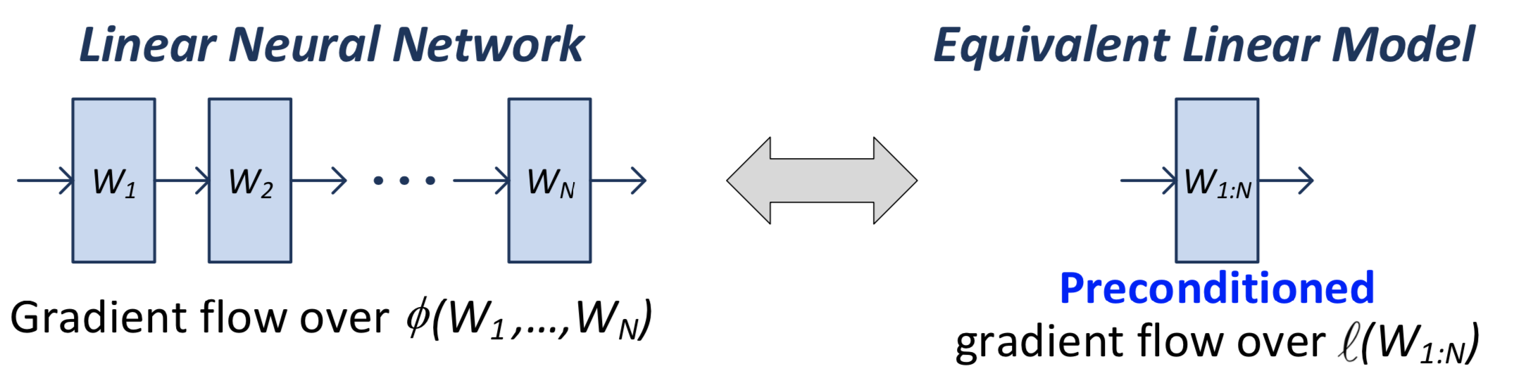
What you can show is that the gradient flow of the \(W_{1:N}\) matrix is equivalent to a pre-conditioned version of the single-layer gradient:
\[ \begin{equation} \frac{d}{dt} \operatorname{vec}\left[ W_{1:N}(t) \right] = - P_{W_{1:N}(t)} \cdot \operatorname{vec}\left[ \nabla l( W_{1:N}(t)) \right] \tag{1} \end{equation} \]
Thus, adding additional (redundant) linear layers induces “preconditioners promoting movement in directions already taken”.[^ Preconditioners are linear transformations that condition a problem to make it more suitable for numerical solutions, and usually involve reducing the condition number. It turns out that the ideal preconditioner is the M-P pseudo-inverse, which we’ve seen before, [[pseudo-inverses-and-sgd]].]
Recall that the condition number is the ratio of the max to the min singular value, so relates to how much the matrix scales the input.
Important: this above analysis (1) is independent of the form of the loss function. I think the only requirement is that the parameters come into the loss function through the end-to-end matrix.
Equivalent Explicit Form?
So, we see that depth plays this role of preconditioning. A question is, does there exist some other loss function \(F\) such that
\[ \begin{equation*} \frac{d}{dt} \operatorname{vec}\left[ W_{1:N}(t) \right] = - P_{W_{1:N}(t)} \cdot \operatorname{vec}\left[ \nabla l( W_{1:N}(t)) \right] = - \operatorname{vec}\left[ \nabla F (W_{1:N}(t)) \right]. \end{equation*} \]
That is, is there just some particularly smart loss function that you could pick that is able to recreate this depth effect? It turns out the answer is no. At this point, we should be talking about the particular matrix completion loss function. The proof involves: by the gradient theorem, we have that, for some closed loop \(\Gamma\),
\[ \begin{align*} 0 = \int_{\Gamma} \operatorname{vec}\left[ \nabla F (W) \right] dW = \int_{\Gamma} P_{W} \cdot \operatorname{vec}\left[ \nabla l(W) \right] dW. \end{align*} \]
Turns out you need some technical details, involving actually constructing a closed loop, the details of which can be found on page 6 of (Arora, Cohen, and Hazan 2018Arora, Sanjeev, Nadav Cohen, and Elad Hazan. 2018. “On the optimization of deep networks: Implicit acceleration by overparameterization.” In 35th International Conference on Machine Learning, Icml 2018, 372–89. Institute for Advanced Studies, Princeton, United States.).
Ultimately, this is not particularly interesting, because a) it’s an exact statement: okay, there’s no explicit choice of loss function that exactly replicates this, but that doesn’t prevent there from being something arbitrarily close; and b) …1 So actually I was going to say that, this is a strawman argument, since they are dealing with an essentially degenerate linear network so clearly you can’t do any better than something like convex programs (and it’s just barely even overparameterized?). But now I’m realizing that we never did depth 1, since it just felt silly. But perhaps depth 1 actually works too. Time to find out…
Optimization
Consider again (1). Murky on the details (see slides), but since \(P_{W:N}(t) \succ 0\), then the loss decreases until \(\nabla l(W_{1:N}(t)) = 0\). Then under certain conditions (\(l\) being convex), this means gradient flow converges to a global minimum.
What this is saying: for arbitrary convex loss function, running a DLNN gives a global minimum. If loss is \(l_2\), you can actually get a linear rate of convergence.
This stuff is pretty cool, simply because gradient descent really shouldn’t have any global guarantees. The only way for you to be able to have global guarantees is if you have some control over the trajectory.
Note though that this doesn’t say anything about generalization performance.