#lit_review
Learning as the Unsupervised Alignment of Conceptual Systems
src: (Roads and Love 2020Roads, Brett D, and Bradley C Love. 2020. “Learning as the unsupervised alignment of conceptual systems.” Nature Machine Intelligence 2 (1): 76–82.)
The surprising thing about * embeddings is that it relies solely on co-occurrence, which you can define however you want. This makes it a powerful generalized tool.1 And more generally, a key insight in statistical NLP is to not worry (too much) about the words themselves (except maybe during the preprocessing step, with things like stemming), but simply treat them as arbitrary tokens. For example, as in this paper, we can consider objects (or captions) of an image, and co-occurrence for objects that appear together in an image. From this dataset (Open Images V4: github), we can construct a set of embedding vectors (using GloVe) for the objects/captions (call this GloVe-img).
What is this set of embeddings? You can think of this as a crude learning mechanism of the world, using just visual data.2 Potential caveat (?): part of the data reflects what people want to take photos of, and be situated together. Though for the most part the objects in the images aren’t being orchestrated, it’s more just what you find naturally together. In other words, if a child were to learn through proximity-based associations alone, then perhaps this would be the extent of their understanding of the world.
A natural followup is, then, how does this embedding compare to the standard GloVe learned from a large text corpus?
At this point, I need to digress and talk about what this paper does:
- take the similarity matrix of the original GloVe vectors and the GloVe-img vectors. calculate the correlation of the matched entries. turns out that correlation can get as high as 0.3. perhaps that’s surprising?
- seems like a waste to project things down to a similarity matrix. on the other hand, the arbitrariness of embeddings might make it difficult to compare embeddings directly.
Judicial Demand for xAI
src: paper, via Michelle.
For the [[project-fairness]], we have been thinking in terms of algorithms and how to better design them to be better vanguards of such societal principles as equality. Something that I hadn’t thought about is the legal side of things; that is, what are the legal raminifications of introducing algorithms (and in the future, more powerful AI) to the legal process? If a judge’s decision rests on the results of an algorithm (e.g. criminal proceedings and giving bail), if lawyers themselves use algorithms for automating tasks (even creation of bills), or if it is the result of the algorithm in question that causes something persecutable (automated drones, self-driving cars) – these are all different examples of how AI might be part of the process.
The COMPAS debacle is a concrete example, and we saw the defendent argue that “the court’s use of the risk assessment violated his due process rights, in part because he was not able to assess COMPAS’s accuracy”. Clearly this is getting into legal territory – namely, what are his due process rights? What is sufficient for him to assess the accuracy?
The paper takes the view that explainable AI (xAI) is the answer to all this, and that it should be the judges (via the process of common law) that ought to decide the nature of the kinds of xAI that should be required depending on the circumstances. I don’t have much to say about the latter aspect of the thesis, as IANAL. However, my feeling is that this is just a much easier problem than the author makes it out to be; namely, just make it so that every algorithm is equipped with a full suite of xAI. It’s really not that difficult, and not much of an onus on the engineers. And one could go so far as require all closed-source algorithms have an open-source alternatives (or, as mentioned in the paper, I’m sure you can use existing legal structures involving confidential material).
This all feels like a red-herring to me though, and sidesteps the crux of the problem, which goes back to what I’ve been working on: the actual equitability or fairness of these algorithms. The idea is that, if you have xAI, and you can see the inner workings, then you can catch it doing bad things (which I agree), but if we’re going to be using algorithms, then we better actually be using justified algorithms before we apply them in court, at which point the xAI part of things is moot. For instance, if you were to show the defendent in the COMPAS example all the deconstructed analysis of the model, even right now there is no consensus among even academics about the fairness of the algorithm, how is this going to help anyone?
Also, the first thing that comes to my mind whenever we talk about xAI is that humans often have a hard time actually explaining their thought process – and yet, that has rarely stopped anyone in court. So part of this, I feel, is more a faith-in-humanity-more-than-machines type argument, which, as long as our prejudices are laid bare, I’m fine with that. Perhaps underlying that line of argument is the reasonableness or rationality of humans versus machines.1 This reminds me of how for self-driving cars, the bar is much higher when it comes to the level of safety before people feel comfortable. There’s this sort of weird disconnect between what we expect from AI, and what we expect from our fellow humans.
Explainable AI
Explainability can come in various forms. The easiest, as it does not require opening the box, are wrapper-type methods that essentially try to describe the function being approximated in terms of something understandable, whether it be things like counterfactuals, or english interpretations of the form of the function. Similarly, one can build surrogate models (e.g. decision trees, linear models) that approximate the function (though you obviously lose accuracy), and provide a better trade-off.2 This approach seems a little weird to me though (and feels a little bit like russian dolls), where you’re basically trading (peeling) off complexity for more simple and interpretable models, but you’re not really comparing apples to oranges at that point.
Here’s an [[idea]]: what if you can come up with something like the tangent plane, but the explainable plane, in that for every point estimate provided by the machine learning model, you can just find a super simple, interpretable model that does a good, local job of explaining stuff for that particular defendent (has to exactly predict what the ML model predicted, hence the parallels to the tangent plane). Actually, this is very similar to LIME (Ribeiro, Singh, and Guestrin 2016Ribeiro, Marco Tulio, Sameer Singh, and Carlos Guestrin. 2016. “"Why Should I Trust You?".” In KDD ’16: The 22nd Acm Sigkdd International Conference on Knowledge Discovery and Data Mining, 1135–44. New York, NY, USA: ACM.).
The other class of methods involve delving into the black-box, and providing method-specific interpretations of the actual learned model (e.g. for things like CNN, you can look at pixel-level heat-maps), or something more naive like just providing the model as a reproducible instance.
Noisy Networks
src: Chang, Kolaczyk, and Yao (2018Chang, Jinyuan, Eric D Kolaczyk, and Qiwei Yao. 2018. “Estimation of subgraph density in noisy networks.” arXiv.org, March. http://arxiv.org/abs/1803.02488v3.), Li, Sussman, and Kolaczyk (2020Li, Wenrui, Daniel L Sussman, and Eric D Kolaczyk. 2020. “Estimation of the Epidemic Branching Factor in Noisy Contact Networks,” February. http://arxiv.org/abs/2002.05763.)
A common task in network analysis is to calculate a network statistic, from which some conclusion can be gleaned. Oftentimes you’ll have a table of typical summary statistics for your graphs, and they can be either (average) node-level statistics (like centrality), or global statistics (like edge density). There is usually not much import to those tables – mainly used just so people can get a feel for the graph/dataset.
Sometimes though you’re interested in some particular real-valued functional of the network. For instance, in my previous work, we were interested in unbalanced triangles. Another statistic, very relevant to #coronavirus, is the branching factor, or \(R_0\), of a contact network (see Li, Sussman, and Kolaczyk (2020Li, Wenrui, Daniel L Sussman, and Eric D Kolaczyk. 2020. “Estimation of the Epidemic Branching Factor in Noisy Contact Networks,” February. http://arxiv.org/abs/2002.05763.) for more details).
Whenever you have a statistic, you might want to know two things: how confident are you of this value, or what is the “variability” of this statistic; and whether or not this statistic is significant. Let’s take this latter approach first. The idea here is that we have some hypothesis that we want to test, and so we need to first construct a null hypothesis, and the statistic is the mechanism (or measure) through which which we can judge the significance of our test. In the former case, all that we really want is just a set of confidence intervals for our statistic. It’s almost the same thing, except there is no hypothesis – all that is required is a random model that lets you define the form of the noise, and therefore construct confidence intervals.
So in fact, there is a subtle difference between these two things. For the most part, I have been thinking about the latter (hypothesis testing), but attaching confidence bands to point estimates in networks is also an interesting research question.
Noise Model
The noise model analyzed in these papers is very straightforward. It essentially follows the paradigmatic signal + noise model in statistics. Fix a graph \(G\) (defined by its adjacency matrix \(A\)), which we think of as the ground truth. Then the noisy observation (adjacency matrix \(\widetilde{A}\)) are produced by random bit-flips (0 to 1 or 1 to 0). For simplicity, the random bit-flips are modelled with only two parameters: \(\alpha\), the Type-1 error, and \(\beta\), the Type-2 error. That is,
\[ \begin{align*} P(\widetilde{A}_{ij} = 1 \given A_{ij} = 0) = \alpha, \quad P(\widetilde{A}_{ij} = 0 \given A_{ij} = 1) = \beta, \end{align*} \]
Thus, you’ve reduced the whole problem to estimating two parameters.1 Which feels a little extreme. Unsurprisingly, you use #method_of_moments to estimate them. However, because you have two parameters, you’re going to need more than one sample (i.e. two).
Actually, I think it’s a little more complicated than that (it’s not really a degree-of-freedom thing). One might think that with a large enough graph, you can probably split in two, and estimate the parameters on each half (and they’d be independent). However, I suspect the problem is that the model is a little too general, so if your \(\alpha, \beta\) are too large, then you can’t really guess anything.2 i.e. you have no control of what’s signal and what’s noise. My guess is that if you have two samples, then you have access to the intersection/set-difference, which makes it more feasible to estimate things. But the thing is that this then relies on the intersection.
This makes me think that a) if you restrict the \(\alpha, \beta\) to be suitably small, then you can probably be okay with one sample; and b) this model is actually pretty restrictive.3 I mean, in terms of the space of possible samples it is fine, but I guess like any model, you really don’t want your results to depend so much on the assumptions.
This is similar to the #stochastic_blockmodel, in that these parameters are really just nuisance parameters. In that model, you can actually estimate many things without actually knowing these nuisance parameters.
Remark. It might seem weird to fix a graph. Clearly I cannot be too against this notion, since the test I propose also assumes a fixed graph. However, in that particular setting, I felt that was the best option. Not something that I thought was particularly realistic (but the alternatives, considering parametric models seemed even more riddled with problems).
In my opinion, this particular model must be considered together with the particular application. A concrete example would be protein networks. I don’t know how these datasets are generated, and so it is unclear to me if such a noise model would be an accurate representation. The key thing here is that this is how we’re modelling the multiple draws/samples.A Better Model?
Two things come to mind. First is model-fitting and checking, though not necessarily singularly focused on this particular noise model. As I’ve said before, almost all network models are a terrible model for real-life data, especially the parametric ones. This particular model is technically parametric, but very different. So what we want are diagnostic checks to see how comformal our data is to the models. Since this procedure utilizes the fact that you have multiple samples, then that also means that you probably should be able to use that for diagnostics.
Along a similar line, it seems that what we would want is a more robust version of this noise model. Or, another way to think about this is that, what you want are estimators that are more robust to the model assumptions.4 like median for measure of centrality not assuming normality in the errors. I’m not really sure what the form of this would be: something a little more non-parametric?
If we are interested in the application of contact networks, then it might be fruitful to consider in isolation, and come up with a particular noise model that we think suits this dataset.5 and potentially the paper could be a general type of paper that we can then demonstrate specializing to different data types.
Matrix Completion Optimization
Let’s try to understand the landscape of optimization in matrix completion.
Matrix Factorization
A celebrated result in this area is (Ge, Lee, and Ma 2016Ge, Rong, Jason D Lee, and Tengyu Ma. 2016. “Matrix completion has no spurious local minimum.” In Advances in Neural Information Processing Systems, 2981–9. University of Southern California, Los Angeles, United States.). They consider the matrix factorization problem (with symmetric matrix, so that it can be written as \(XX^\top\)). Note that this problem is non-convex.1 The general version of this problem, with \(UV^\top\), interestingly, is at least alternatingly (marginally) convex (which is why people do alternating minimization). Under some typical incoherence conditions,2 To ensure that there is enough signal in the matrix, preventing cases where all the entries are zero, say. they are able to show that this optimization problem has no spurious local minima. In other words, for every optima to the function \[ \begin{align*} \widetilde{g}(x) = \norm{ P_\Omega (M - X X^\top) }_F^2, \end{align*} \] it is also a global minima (which means \(=0\)).3 They were inspired, in part, by the empirical observation that random initialization sufficed, even though all the theory required either conditions on the initialization, or some more elaborate procedure.
Proof technique: they compare this sample version \(\widetilde{g}(x)\) to the population version \(g(x) = \norm{ M - X X^\top }_F^2\), and use statistics and concentration equalities to get desired bounds.
Remark. The headline (no spurious minima) sounds amazing, but it’s not actually that non-convex. In any case, as it turns out, it’s basically non-convex (i.e. multiple optima) because you have identifiability issues with orthogonal rotations of the matrix (that cancel in the square). I wonder if the incoherence condition is important here. I don’t think so, as it’s a pretty broad set, so it really does seem like this problem is pretty well-behaved.
A nice thing about the factorization is that zero error basically means you’re done (given some conditions on sample size), since having something that factorizes and gets zero error must be the low-rank answer.To reiterate, they don’t use any explicit penalty (except something that’s helpful for the proof technique to ensure you are within the coherent regime). The matrix factorization form suffices.
Important: something I missed the first time round, but actually makes this somewhat less impressive: they basically assume the rank is given, and then force the matrix to have that dimension. This differs from (Arora et al. 2019Arora, Sanjeev, Nadav Cohen, Wei Hu, and Yuping Luo. 2019. “Implicit Regularization in Deep Matrix Factorization.” arXiv.org, May. http://arxiv.org/abs/1905.13655v3.)’s deep matrix factorization as there they aren’t forcing the dimensions. This doesn’t seem that impressive anymore.
Non-Convex Optimization
src: off-convex.
The general non-convex optimization is an NP-hard problem, to find the global optima. But even ignoring the problem of local vs global, it’s even difficult to differentiate between optima and saddle points.
Saddle points are those where the gradients in the direction of the axis happen to be zero (usually one is max, the other is a min). In the case of gradient descent, since we move in the direction of gradient for each coordinate separately, then we’re basically stuck.
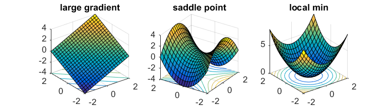
If one has access to second-order information (i.e. the Hessian), then it is easy to distinguish minima from saddle points (the Hessian is PSD for minima). However, it is usually too expensive to calculate the Hessian.
What you might hope is that the saddle points in the problem are somewhat well-behaved: there exists (at least) one direction such that the gradient is pretty steep. This way, if you can perturb your gradient, then hopefully you’ll accidentally end up in that direction that lets you escape it.
That’s where noisy gradient descent (NGD) comes into play. This is actually a little different to stochastic gradient descent, which is noisy, but that noise is a function of the data. What we want is actually to perturb the gradient itself, so you just add a noise vector with mean 0. This allows the algorithm to effectively explore all directions.4 In subsequent work, it has been established that gradient descent can still escape saddle points, but asymptotically, and take exponential time. On the other hand, NGD can solve it in polynomial time.
What they show is that NGD is able to escape those saddle points, as they eventually find that escape direction. However, the addition of the noise might have problems with actual minima, since it might perturb the updates sufficiently to push it out of the minima. Thankfully, they show that this isn’t the case. Intuitively, this feels like it shouldn’t be that hard – if you imagine a marble on these surfaces, then it feels like it should be pretty easy to perturb oneself to escape the saddles, while it seems fairly difficult to get out of those wells.
Proof technique: replace \(f\) by its second-order taylor expansion \(\hat{f}\) around \(x\), allowing you to work with the Hessian directly. Show that function value drops with NGD, and then show that things don’t change if you go back to \(f\). In order for this to hold, you need the Hessian to be sufficiently smooth; known as the Lipschitz Hessian condition.
It turns out that it is relatively straightforward to extend this to a constrained optimization problem (since you can just write the Lagrangian form which becomes unconstrained). Then you need to consider the tangent and normal space of this constrain set. The algorithm is basically projected noisy gradient descent (simply project onto the constraint set after each gradient update).
Exponential Learning Rates
via blog and (Li and Arora 2019Li, Zhiyuan, and Sanjeev Arora. 2019. “An Exponential Learning Rate Schedule for Deep Learning.” arXiv.org, October. http://arxiv.org/abs/1910.07454v3.)
Two key properties of SOTA nets: normalization of parameters within layers (Batch Norm); and weight decay (i.e \(l_2\) regularizer). For some reason I never thought of BN as falling in the category of normalizations, ala [[effectiveness-of-normalized-quantities]].
It has been noted that BN + WD can be viewed as increasing the learning rate (LR). What they show is the following:
The proof holds for any loss function satisfying scale invariance: \[ \begin{align*} L(c \cdot \theta) = L(\theta) \end{align*} \] Here’s an important Lemma:
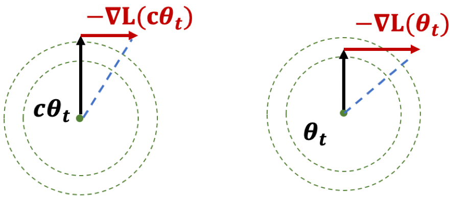 Figure 1: Illustration of Lemma
The first result, if you think of it geometrically (Fig. 1), ensures that \(|\theta|\) is increasing. The second result shows that while the loss is scale-invariant, the gradients have a sort of corrective factor such that larger parameters have smaller gradients.
Thoughts
The paper itself is more interested in learning rates. What I think is interesting here is the preoccupation with scale-invariance. There seems to be something self-correcting about it that makes it ideal for neural network training. Also, I wonder if there is any way to use the above scale-invariance facts in our proofs.
They also deal with learning rates, except that the rates themselves are uniform across all parameters, make it much easier to analyze—unlike Adam where you have adaptivity.
Does Learning Require Memorization?
src: (Feldman 2019Feldman, Vitaly. 2019. “Does Learning Require Memorization? A Short Tale about a Long Tail.” arXiv.org, June. http://arxiv.org/abs/1906.05271v3.)
A different take on the interpolation/memorization conundrum.
The key empirical fact that this paper rests on is this notion of data’s long-tail.1 This was all the rage back in the day, with books written about it. Though that was more about #economics and how the internet was making it possible for things in the long tail to survive. Formally, we can break a class down into subpopulations (say species2 Though they don’t have to be some explicit human-defined category.), corresponding to a mixture distribution with decaying coefficients. The point is that this distribution follows a #power_law distribution.
Now consider a sample from this distribution (which will be our training data). You essentially have three regimes:
- Popular: there’s a lot of data here, you don’t need to memorize, as you can take advantage of the law of large numbers.
- Extreme Outliers: this is where the actual population itself is already incredibly rare, so it doesn’t really matter if you get these right, since these are so uncommon.
- Middle ground: this is middle ground, where you still might only get one sample from this subpopulation, but it’s just common enough (and there are enough of them) that you want to be right. And since they’re uncommon, you basically only have one copy anyway, so your best choice is to memorize.
Key: a priori you don’t know if your samples are from the outlier, or from the middle ground. So you might as well just memorize.3 What you have is that actually, what you don’t mind is selective memorization. Though it’s probably too much work to have two regimes, so just memorize everything.
My general feeling is that there is probably something here, but it feels a little too on the nose. It basically reduces the power of deep learning to learning subclasses well, when I think it’s more about the amalgum of the whole thing.
Relation to DP
Here’s an interesting relation to #differential_privacy. One of the motivations for this paper is that DP models (DP implies you can’t memorize) fail to achive SOTA results for the same problem as these memorizing solutions. If you look at how these DP models fail, you see that they fail on the exact class of problems as those proposed here, i.e. it cannot memorize the tail of the mixture distribution. This is definitely something to keep in mind for [[project-interpolation]].
Benign Overfitting in Linear Regression
src: (Bartlett et al. 2020Bartlett, Peter L, Philip M Long, Gábor Lugosi, and Alexander Tsigler. 2020. “Benign overfitting in linear regression.” Proceedings of the National Academy of Sciences of the United States of America vol. 80 (April): 201907378.).
- references:
- setting:
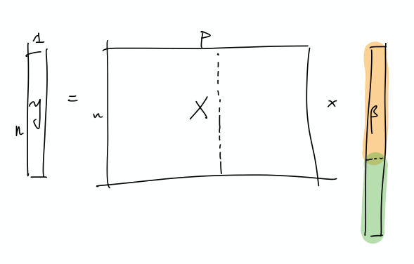
- linear regression (quadratic loss), linear prediction rule
- important: we are actually thinking about the ML regime, whereby there isn’t just a true parameter, but that there is a best one by considering the expectation (which, under general settings, corresponds to what would be the “truth”).
- important: they are considering random covariates in their analysis! I guess this is pretty standard practice, when you’re calculating things like risk
- that is, you can think of linear regression as a linear approximation to \(\mathbb{E} ( Y_i \,\mid\, X_i)\)
- blog with a good explanation: very standard classical exposition, showing that the conditional expectation is the optimal choice for \(L_2\) loss, and the linear regression solutions is the best linear approximation to the conditional expectation (something like that)
- infinite dimensional data: \(p = \infty\) (separable Hilbert space)
- though results apply to finite-dimensional
- thus, there exists \(\theta^*\) that minimizes the expected quadratic loss
- in order to be able to calculate expected value, they must be assuming some model (normal error)
- but they want to deal with the interpolating regime, so at the very least \(p > n\), and probably >>
- “We ask when it is possible to fit the data exactly and still compete with the prediction accuracy of \(\theta^*\).”
Unless I’m being stupid, this line doesn’t make any sense. If you fit the data exactly, then by definition you’re an optimal solution
- the solution that minimizes is underdetermined, so there isn’t a unique solution to the convex program
- okay, so I think what they’re trying to say is that, if your choice of \(\hat{\theta}\) is the one that minimizes the quadratic loss (= 0), and then pick the one with minimum norm (what norm), then let’s see when do you get good generalizability
- “We ask when it is possible to overfit in this way – and embed all of the noise of the labels into the parameter estimate \(\hat{\theta}\) – without harming prediction accuracy”
- linear regression (quadratic loss), linear prediction rule
- results:
- covariance matrix \(\Sigma\) plays a crucial role
- prediction error has following decomposition (two terms):
- provided nuclear norm of \(\Sigma\) is small compared to \(n\), then \(\hat{\theta}\) can find \(\theta^*\)
- impact of noise in the labels on prediction accuracy (important)
- “this is small iff the effective rank of \(\Sigma\) in the subspace corresponding to the low variance directions is large compared to \(n\)”
- “fitting the training data exactly but with near-optimal prediction accuracy occurs if and only if there are many low variance (and hence unimportant) directions in parameter space where the label noise can be hidden”
- intuition: I don’t think they’ve provided much in the way of any intuition about what is going on, so let’s see if we can come up with some
- this is weird because we’re thinking of linear regression, and so basically it’s a linear combination of the \(X\)’s to get \(Y\).
- if we were to think about this geometrically, is that we have an infinite dimensional \(C(X)\), with sufficient “range”/span that our \(Y\) lands in \(C(X)\).
- I feel like what they’re trying to do is basically have the main true linear model, and then what you have are these small vectors in all sorts of directions, so that you can just add those to your solution, in order to interpolate (??)
- and since we’re dealing with a model that is linear in truth, then
- I’m confused, because since both \(x,y\) are random, then calculating the risk is over both of these things.
- takeaway:
- basically, the eigenvalues of the covariance matrix should satisfy:
- many non-zero entries, large compared to \(n\)
- small sum compared to \(n\) (smallest eigenvalues decays slowly)
- i.e. lots of small ones, probably some big ones (?)
- basically, the eigenvalues of the covariance matrix should satisfy:
- summary: this is what I think is going on
- let’s just start with \(X\) and it’s covariance matrix \(\Sigma\): what we have here is something, at the population level, that can be described by a few large eigenvalues, and then many, many small eigenvalues. The idea is that the \(\Sigma\) describes the distribution of the sampled \(x\) vectors, and so the eigenvalues determine the variability in the direction of the respective engeinvector. However, there is no guarantee that there needs to be a rotation, so it is entirely possible that the variability in the \(x\)’s are concentrated on individual coordinates.
I incorrectly thought that what we have are random vectors, and so this spans all the coordinates, which makes it easier to extract the coefficients
- So what we need are very many small directions of \(x\) (again, you can just align them to a coordinate)…
- The optimal thing would be this nice sort of decomposition, where the first few elements of \(\beta\) correspond to the true coefficients. Then, the point is that the error can be entirely captured by a linear combination of the rest of the covariates.
- This is a more explicit decomposition of the two terms
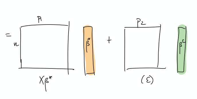
- The idea here is that, in some simplified sense, the error is just a random Gaussian vector, and we should be able to represent it exactly as a linear combination of a lot of small gaussian vectors.
- let’s just start with \(X\) and it’s covariance matrix \(\Sigma\): what we have here is something, at the population level, that can be described by a few large eigenvalues, and then many, many small eigenvalues. The idea is that the \(\Sigma\) describes the distribution of the sampled \(x\) vectors, and so the eigenvalues determine the variability in the direction of the respective engeinvector. However, there is no guarantee that there needs to be a rotation, so it is entirely possible that the variability in the \(x\)’s are concentrated on individual coordinates.
Backlinks
- [[pseudo-inverses-and-sgd]]
- thanks to this tweet, realize there’s a section in (Zhang et al. 2019Zhang, Chiyuan, Benjamin Recht, Samy Bengio, Moritz Hardt, and Oriol Vinyals. 2019. “Understanding deep learning requires rethinking generalization.” In 5th International Conference on Learning Representations, Iclr 2017 - Conference Track Proceedings. University of California, Berkeley, Berkeley, United States.) [[rethinking-generalization]] that relates to (Bartlett et al. 2020Bartlett, Peter L, Philip M Long, Gábor Lugosi, and Alexander Tsigler. 2020. “Benign overfitting in linear regression.” Proceedings of the National Academy of Sciences of the United States of America vol. 80 (April): 201907378.) [[benign-overfitting-in-linear-regression]], in that they show that the SGD solution is the same as the minimum-norm (pseudo-inverse)
- the curvature of the minimum (LS) solutions don’t actually tell you anything (they’re the same)
- “Unfortunately, this notion of minimum norm is not predictive of generalization performance. For example, returning to the MNIST example, the \(l_2\)-norm of the minimum norm solution with no preprocessing is approximately 220. With wavelet preprocessing, the norm jumps to 390. Yet the test error drops by a factor of 2. So while this minimum-norm intuition may provide some guidance to new algorithm design, it is only a very small piece of the generalization story.”
- but this is changing the data, so I don’t think this comparison really matters – it’s not saying across all kinds of models, we should be minimizing the norm. it’s just saying that we prefer models with minimum norm
- interesting that this works well for MNIST/CIFAR10
- there must be something in all of this: on page 29 of slides, they show that SGD converges to min-norm interpolating solution with respect to a certain kernel (so the norm is on the coefficients for each kernel)
- as pointed out, this is very different to the benign paper, as this result is data-independent (it’s just a feature of SGD)
- thanks to this tweet, realize there’s a section in (Zhang et al. 2019Zhang, Chiyuan, Benjamin Recht, Samy Bengio, Moritz Hardt, and Oriol Vinyals. 2019. “Understanding deep learning requires rethinking generalization.” In 5th International Conference on Learning Representations, Iclr 2017 - Conference Track Proceedings. University of California, Berkeley, Berkeley, United States.) [[rethinking-generalization]] that relates to (Bartlett et al. 2020Bartlett, Peter L, Philip M Long, Gábor Lugosi, and Alexander Tsigler. 2020. “Benign overfitting in linear regression.” Proceedings of the National Academy of Sciences of the United States of America vol. 80 (April): 201907378.) [[benign-overfitting-in-linear-regression]], in that they show that the SGD solution is the same as the minimum-norm (pseudo-inverse)
- [[matrix-factorization-to-linear-model]]
- Update: following on from [[experimental-logs-for-matrix-completion]], we have looked at how the nuclear norm fails in the depth-1 case, which is that you dampen the top singular values and reconstruct the residuals from small singular vectors (feels ever so slightly like [[benign-overfitting-in-linear-regression]]).
Nonparametric Testing on Graphs
Lit Review
- Testing Equivalence of Clustering, (Gao and Ma 2019Gao, Chao, and Zongming Ma. 2019. “Testing Equivalence of Clustering.” arXiv.org, October. http://arxiv.org/abs/1910.12797v2.)
- abstract
- “In this paper, we test whether two datasets share a common clustering structure. As a leading example, we focus on comparing clustering structures in two independent random samples from two mixtures of multivariate Gaussian distributions. Mean parameters of these Gaussian distributions are treated as potentially unknown nuisance parameters and are allowed to differ. Assuming knowledge of mean parameters, we first determine the phase diagram of the testing problem over the entire range of signal-to-noise ratios by providing both lower bounds and tests that achieve them. When nuisance parameters are unknown, we propose tests that achieve the detection boundary adaptively as long as ambient dimensions of the datasets grow at a sub-linear rate with the sample size.”
- abstract
- Minimax Rates in Network Analysis: Graphon Estimation, Community Detection and Hypothesis Testing, (Gao and Ma 2018Gao, Chao, and Zongming Ma. 2018. “Minimax Rates in Network Analysis: Graphon Estimation, Community Detection and Hypothesis Testing.” arXiv.org, November. http://arxiv.org/abs/1811.06055v2.)
- tests involving ER vs SBM
- more general test that handle “degree-corrected” i’m guessing (via his paper with Lafferty)
- results in a nice test that involves counts of subgraphs/motifs (essentially boiling down to edges, vees and triangles)
- it’s independent of the heterogeneity of the degree distribution, so you don’t have to estimate those nuisance parameters
- Network Global Testing by Counting Graphlets (Jin, Ke, and Luo 2018Jin, Jiashun, Zheng Tracy Ke, and Shengming Luo. 2018. “Network Global Testing by Counting Graphlets.” arXiv.org, July. http://arxiv.org/abs/1807.08440v1.)
- reminds me of the method-of-moments type thing we did in the [[parameter-estimation-in-sbm]] paper
Backlinks
- [[master-paper-list]]
- [[nonparametric-testing-on-graphs]] (this could also be a more applied paper, that discusses the general problem with doing tests, or just modeling things in social networks)
- JASA
- [[nonparametric-testing-on-graphs]] (this could also be a more applied paper, that discusses the general problem with doing tests, or just modeling things in social networks)
Matrix Completion Optimal Rates
Literature Review
Candes and Plan (2009Candes, Emmanuel J, and Yaniv Plan. 2009. “Matrix Completion with Noise.” Proceedings of the IEEE 98 (6): 925–36.) :
RMS: \(\dfrac{\norm{\hat{M} - M}_{F}}{N}\)
Oracle rate: \[ \begin{equation} \norm{ M^{*} - M }_{F} \approx p^{-1/2} \delta, \tag{1} \end{equation} \] where \(\delta = \norm{Z}_{F}\), \(Z\) is the added noise matrix, and \(p = \frac{m}{n^2}\) is the fraction of observed entries1 Something weird: this obviously breaks down when \(\delta = 0\), or if it has to be positive, then just take the limit.. This is for arbitrary noise. When it’s white (with s.d. \(\sigma\)), then \[ \norm{ M^{*} - M }_{F} \approx \sqrt{\frac{nr}{p}} \sigma, \] where \(r\) is the rank of the low-rank matrix. To translate this into \(\delta\), we have \(\E{\delta} = \E{\norm{F}_{Z}} \approx n \sigma\), and so RHS is \(\sqrt{\frac{r}{np}} \delta\). Comparing this to (1), this is much sharper since \(r\) is very small.
Their method (which uses some form of SDP) seem to get something like \(\sqrt{n}\) off the oracle rate.
Negahban and Wainwright (2012Negahban, Sahand, and Martin J Wainwright. 2012. “Restricted strong convexity and weighted matrix completion: Optimal bounds with noise.” Journal of Machine Learning Research 13 (May): 1665–97.) :
error is scaled here by \(\frac{\eta}{d_r d_c} = \frac{\sigma}{n^2}\), so that it’s independent of the ambient dimension.
they actually use our ratio, not to regularize, but to “provide a tractable measure of how close \(\Omega\) is to a low-rank matrix”.
Hastie et al. (2015Hastie, Trevor, Rahul Mazumder, Jason Lee, and Reza Zadeh. 2015. “Matrix completion and low-rank SVD via fast alternating least squares,” January.) : this is SoftImpute.
they make the comparison between (Cai, Candes, and Shen 2010Cai, Jian-Feng, Emmanuel J Candes, and Zuowei Shen. 2010. “A Singular Value Thresholding Algorithm for Matrix Completion.” SIAM Journal on Optimization 20 (4): 1956–82.), which essentially solves \[ \begin{equation} \min \norm{Z}_{*} \text{ s.t. } P_{\Sigma}(Z) = P_{\Sigma}(X), \tag{2} \end{equation} \] compared to the noisy relaxed version in this paper: \[ \begin{align*} \min \norm{Z}_{*} \text{ s.t. } \norm{P_{\Sigma}(Z) - P_{\Sigma}(X)}_{F} < \delta. \end{align*} \]
Cai, Candes, and Shen (2010Cai, Jian-Feng, Emmanuel J Candes, and Zuowei Shen. 2010. “A Singular Value Thresholding Algorithm for Matrix Completion.” SIAM Journal on Optimization 20 (4): 1956–82.) :
- they propose a first-order method for solving matrix completion that’s very fast and uses little memory
- as it’s iterative, they have a convergence proof
- they also show that the iterates have non-decreasing rank
- this is mainly an engineering task, in that they care about the ability to solve large-scale matrix completion problems (like the Netflix challenge)
Recht (2011Recht, Benjamin. 2011. “A Simpler Approach to Matrix Completion” 12 (104): 3413–30.) :
they show optimality of the convex program (minimizing the nuclear norm, a la (2)), provided \[m > 32 \mu_1 \cdot r n \beta \log^2(n),\] for some \(\beta > 1\) and \(\mu_1\) is something like an upper bound on the entries of singular vectors. they’re not interested in noise, just recovery.
Matrix Factorization
I guess more generally, if you don’t have a square matrix, then the SVD deccomposition is no longer as regular. But that doesn’t seem to be that interesting of a generalization. In any case, iterative methods are often employed, but they suffer from the fact that oftentimes it’ll be biased towards one of the optimization variables (i.e. \(U\) vs \(V\)).
useful links: