#mathematics
Fractals
src: talk at Microsoft Research
Nature vs Culture
Scale-free, or scale-invariance. If you’re given a picture of some rock, then you can’t tell what scale it is at, since you have self-similarity across scaling. Hence you need that reference scale on the bottom right. I wonder if this relates to scale-invariance (à la [[effectiveness-of-normalized-quantities]]).
Roughness. Self-similarity. Now there’s a mathematical framework for thinking about these very human, imprecise notions.1 Curiously, this reminds me of how I think about social networks and how a lot of this messiness is due to social agents. Somehow with this framework it almost seems to abstract away the messiness, and focus on some curious scale-invariance.
Graphs of stock prices have a similar issue (definitely felt this first-hand), whereby if you’re not given time scales, you really can’t distinguish between day or month (besides the upward trend for, say, S&P500).
Independence vs Uncorrelated: if you look at stocks, and if there is a spike one day, then it’s pretty likely that in the next day, there’s also going to be spikes (volatility is high). The only thing is that you don’t know the sign of the activity. So you have expectation zero, but these two events not independent.
Classical take on stock markets is to treat it like brownian motion (continuous time gaussian process). But this doesn’t capture fat-tail-ness and long-range dependence. But with the fractal view, using one parameter (with two real-valued parts), you can basically describe the whole gamut of stock market fluctuations. You can elicit things like anti-persistence and persistence. Start with a trend (upward), add a generator, and then just keep repeating (i.e. fractal).2 Definitely feels like the way you can get brownian motion as a limit to finite random walks, except the key thing is that you’re not taking step sizes to zero, but something a little more self-similar.
- keep moments finite, because then you can take central limit theorems. so things can average out.
The fractal view of markets is descriptive, not prescriptive.
It’s sort of interesting that, with the advent of ML, what you want is over-parameterization. Like that’s sought after now. Whereas in the old days, it’s all about finding the simple thing that then produces complexity. So here Mandelbrot talks about how using multi-fractals, he ends up with only two parameters, and by varying only those two, is able to produce remarkably different scenarios. He contrasts this to other methods, that would have to imbue their model with various extensions in order to be able to capture all the various facets of the characteristics of the price movement.
In some sense, this is good: there seems to be some scale-free nature to price movements. So there is some pattern going on. I’m not too familiar with the math, but I feel like specifying the roughness is half the battle. Or you just say that the rest is just noise or perturbations.
Pseudo-inverses and SGD
- The Moore-Penrose pseudo inverse (which is often just called the pseudoinverse) is just a choice of multiple solutions that leads to a minimum norm solution
- \(\hat{\beta} = X^+ Y\)
- An obvious consequence, is that ridge regression is not the same as the pseudoinverse solution, even though they’re obviously very similar
- my feeling is that, for a particular choice of penalty, the solution should be same (since you should be able to reframe the optimization into
- \(\min ||\beta||_2 \text{ s.t. } ||Y - X \beta ||_2 \leq t\)
- part of me is a little confused: if you can just define this pseudoinverse, then how come we don’t use this estimator more often? clearly it must not have good properties?
- thanks to this tweet, realize there’s a section in (Zhang et al. 2019Zhang, Chiyuan, Benjamin Recht, Samy Bengio, Moritz Hardt, and Oriol Vinyals. 2019. “Understanding deep learning requires rethinking generalization.” In 5th International Conference on Learning Representations, Iclr 2017 - Conference Track Proceedings. University of California, Berkeley, Berkeley, United States.) [[rethinking-generalization]] that relates to (Bartlett et al. 2020Bartlett, Peter L, Philip M Long, Gábor Lugosi, and Alexander Tsigler. 2020. “Benign overfitting in linear regression.” Proceedings of the National Academy of Sciences of the United States of America vol. 80 (April): 201907378.) [[benign-overfitting-in-linear-regression]], in that they show that the SGD solution is the same as the minimum-norm (pseudo-inverse)
- the curvature of the minimum (LS) solutions don’t actually tell you anything (they’re the same)
- “Unfortunately, this notion of minimum norm is not predictive of generalization performance. For example, returning to the MNIST example, the \(l_2\)-norm of the minimum norm solution with no preprocessing is approximately 220. With wavelet preprocessing, the norm jumps to 390. Yet the test error drops by a factor of 2. So while this minimum-norm intuition may provide some guidance to new algorithm design, it is only a very small piece of the generalization story.”
- but this is changing the data, so I don’t think this comparison really matters – it’s not saying across all kinds of models, we should be minimizing the norm. it’s just saying that we prefer models with minimum norm
- interesting that this works well for MNIST/CIFAR10
- there must be something in all of this: on page 29 of slides, they show that SGD converges to min-norm interpolating solution with respect to a certain kernel (so the norm is on the coefficients for each kernel)
- as pointed out, this is very different to the benign paper, as this result is data-independent (it’s just a feature of SGD)
Backlinks
- [[linear-networks-via-gd-trajectory]]
- Thus, adding additional (redundant) linear layers induces “preconditioners promoting movement in directions already taken”.[^ Preconditioners are linear transformations that condition a problem to make it more suitable for numerical solutions, and usually involve reducing the condition number. It turns out that the ideal preconditioner is the M-P pseudo-inverse, which we’ve seen before, [[pseudo-inverses-and-sgd]].]
Power Tower
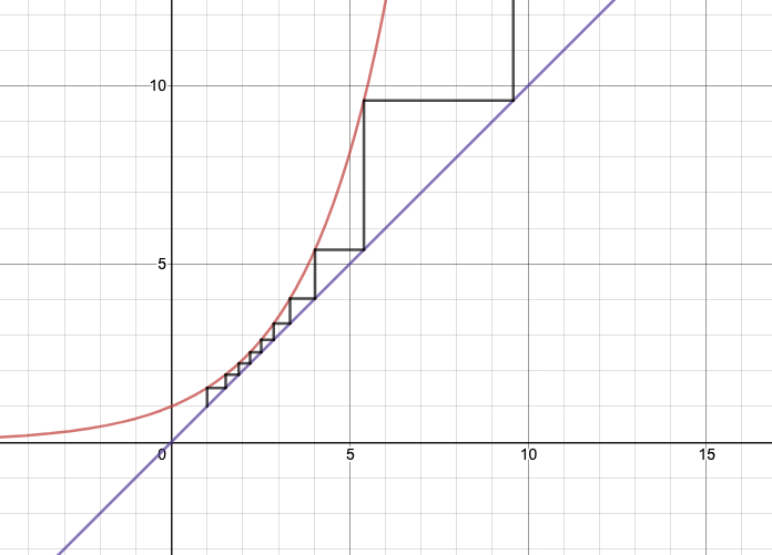 Figure 1: Power Tower for \(b = 1.52\)
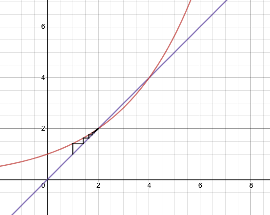 Figure 2: Power Tower for \(b = 2^{1/2}\)
- very simple but cool mathematics: consider the power tower \(x^{x^{x^x}}\)
- for \(x=2\), this blows up at the 6th iteration
- what about for \(x=1.1\)?
- my intuition was that this would also blow up pretty quickly, but nope.
- it basically stabilizes:
- solve \(x^{x^{\cdot^{\cdot^{\cdot}}}} = y\) for some constant \(y\), where \(x = 1.1\)
- note that by the property of \(\infty\), we have \(1.1^y = y\)
- so the limiting factor is the solution to that equation.
- if \(y=4\), what value of \(x\) converges to that?
- \(x^4 = 4 \implies x = \sqrt{2}\).
- but what about \(y=2\)?
- \(x^2 = 2 \implies x = \sqrt{2}\)…as well. oops.
- solve \(x^{x^{\cdot^{\cdot^{\cdot}}}} = y\) for some constant \(y\), where \(x = 1.1\)
- to see what’s going on, just look at Figure 1
- using the cobweb, which is a way to get a progression:
- \(a_0 = 1, a_i = b^{a_{i-1}}\)
- depending on the value of \(b\) (which defines the \(y=b^x\) graph), you’re going to get different behaviour
- the fun thing is that you can’t really tell this unless you draw the graph
- using the cobweb, which is a way to get a progression:
- in particular this (Figure 2) explains the weird thing that happens at \(\sqrt{2}\)
- the reason it doesn’t work is that when you set \(y=4\), and do the substitution of the power-tower on itself, that operation only works if it exists, but it doesn’t, so it’s illegal.
- if you could somehow do it in reverse, then you’d get the \(y=4\), maybe.
New Linear Algebra
New way to teach linear algebra.
\[ \begin{align*} Ax = \begin{bmatrix} 1 & 4 & 5 \\ 3 & 2 & 5 \\ 2 & 1 & 3 \end{bmatrix} \begin{bmatrix} x_1 \\ x_2 \\ x_3 \end{bmatrix} = \begin{bmatrix} 1 \\ 3 \\ 2 \end{bmatrix} x_1 + \begin{bmatrix} 4 \\ 2 \\ 1 \end{bmatrix} x_2 + \begin{bmatrix} 5 \\ 5 \\ 3 \end{bmatrix} x_3 \end{align*} \]
- \(Ax\) is basically a linear combination of the columns
- column space \(C(A)\) is the space spanned by the (3) columns, though since the first two columns add up to the second, it’s just two vectors (rank 2).
\(A = CR\)
\[ \begin{align*} A = CR = \begin{bmatrix} 1 & 4 \\ 3 & 2 \\ 2 & 1 \end{bmatrix} \begin{bmatrix} 1 & 0 & 1 \\ 0 & 1 & 1 \end{bmatrix} \end{align*} \]
- getting independent columns, which is the basis for the column space.
- clearly, you can always do this
- it’s just that sometimes it’s not interesting (i.e. if it’s already a basis)
- \(R\) is the basis for the row space, also rank 2
- number of independent columns = \(r\) = number of independent rows
- \(\operatorname{rank}(C(A)) = \operatorname{rank}(R(A))\)
- \(Ax = 0\) has one solution, and there are \(n-r\) independent solutions to \(Ax = 0\)
- \(R\) turns out to be the row reduced echolon form of \(A\)
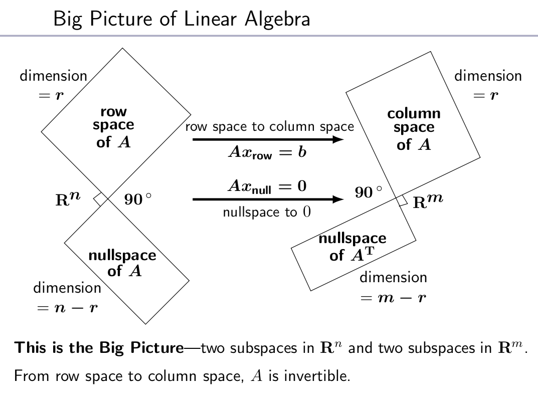
\(Ax = 0\)
\[ \begin{align*} \begin{bmatrix} \text{row } 1 \\ \vdots \\ \text{row } m \end{bmatrix} \begin{bmatrix} \\ x \\ \, \end{bmatrix} = \begin{bmatrix} 0 \\ \vdots \\ 0 \end{bmatrix} \end{align*} \]
- 0 on the right means that the rows must all be orthogonal to \(x\)
- i.e. every \(x\) in the nullspace \(N(A)\) must be orthogonal to the row space.
- if you take transposes you get the equivalent statement for column space
Figure 1: Big Picture Linear Algebra
\(A = BC\)
\[ \begin{align*} A = BC = b_1 c_1^* + b_2 c_2^* + \ldots \end{align*} \]
- here, \(b_i\) are the column vectors of \(B\), while \(c_i^*\) are the row vectors of \(C\).
- you can think of matrix also as column by row multiplication
- it’s more like building blocks there, adding up rank 1 matrices
\(A = LU\)
- you can rewrite \(A\) as a product of lower-triangular and upper-triangular matrices.
- that’s what you’re doing when you’re solving simultaneous equations by elimination
\(Q^\top Q\)
- \(Q\) with orthogonal(normal) column vectors, such that \(Q^\top Q = I\)
- not necessarily true that \(QQ^\top = I\), if not square
- \(QQ^\top\) is like projection:
- \(QQ^\top QQ^\top = QQ^\top\)
- if square, then \(QQ^\top = I\) and \(Q^\top = Q^{-1}\)
- length is preserved by \(Q\)
\(A=QR\)
- Gram-Schmidt: orthogonalize the columns of \(A\).
- assuming full rank of \(C(A)\)
- \(Q^\top A = Q^\top Q R = R\)
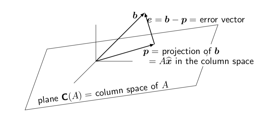
- Major application: Least Squares
- want to minimize \(\norm{b - Ax}^2 = \norm{e}^2\)
- normal equation for minimizing solution (best \(\hat{x}\)): \(A^\top e = 0\)
- if \(A = QR\), then you get \(R \hat{x} = Q^\top b\)
Figure 2: Least Square
\(S = Q \Lambda Q^\top\)
- symmetric matrix \(S=S^\top\) have orthogonal eigenvectors
- how to show \(x^\top y = 0\)
- \(Sx=\lambda x \implies x^\top S^\top = \lambda x^\top \implies x^\top S y = \lambda x^\top y\)
- \(Sy=\alpha y \implies x^\top S y = \alpha x^\top y\)
- hence, \(\lambda x^\top y = \alpha x^\top y\). but \(\lambda \neq \alpha\), since eigenvalues are distinct
- hence, \(x^\top y = 0\)
- things are not nice when things aren’t square
- but \(A^\top A\) is always square, symmetric, PSD
- same holds for \(AA^\top\)
- same eigenvalues
- \(x \to Ax\) to convert eigenvectors
- from definition of eigenvalues: \(AX = X \Lambda\)
- if you don’t have symmetry, then you can’t just hit it with \(X^\top\) and get things to cancel
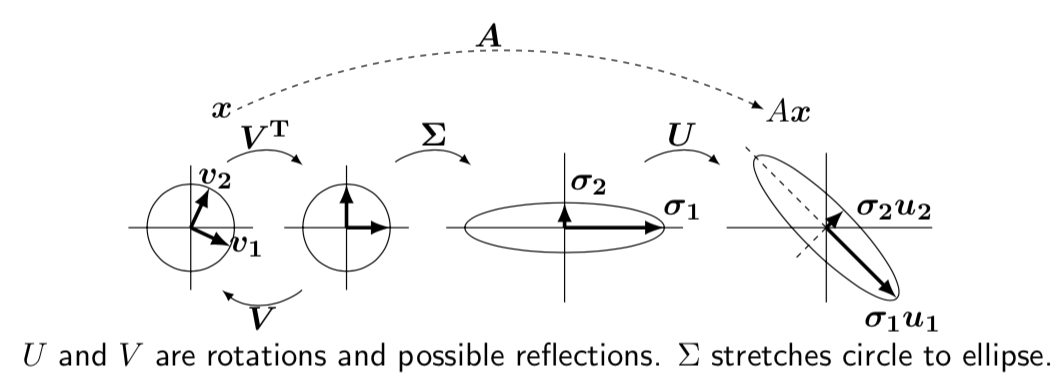
\(A = U \Sigma V^\top\)
- \(U^\top U = I, V^\top V = I\)
- \(AV = U \Sigma\) (like the eigen-decomposition, but not quite)
- \(Av_i = \sigma_i u_i\)
- \(U, V\) are rotations, \(\Sigma\) stretch.
- how to choose orthonormal \(v_i\) in the row space of \(A\)
- \(v_i\) are eigenvectors of \(A^\top A\) (which are orthonormal, from above)
- \(A^\top A v_i = \lambda_i v_i = \sigma_i^2 v_i\)
- so then \(A^\top A V = \Sigma^2 V\)
- how to choose \(u_i\)
- \(u_i = \frac{1}{\sigma_i} A v_i\)
- check orthonormal: \(u_i^\top u_j\)
- combining, \(A^\top A v_i = \sigma_i^2 v_i \implies A^\top u_i = \sigma_i v_i\)
Figure 3: Singular Value Decomposition