#matrix_completion
Experimental Logs for MovieLens
Summary: many of the interesting patterns/phenomena that we see in the noiseless MC case (synthetic data) do not translate when we move to real-life data.1 What’s interesting is that part of me wants to argue like a theoretician, and say that it doesn’t really matter that it doesn’t work on real-life problems. It is slightly different to the way theoretical statistics works, because there the statistical models are usually motivated by solving some real-world problem (though again the same could be said for collaborative filtering). But somehow this feels a little different, as the low-rank matrix problem is a much more general problem than the optimal estimation rates of a particular statistical model. And plus we don’t actually make any claims about the noisy model. The simple answer is that the noisy problem is equalizing, and makes the problem almost trivial (?); that or the fact that the problem isn’t actually that low-rank, so it’s moot to run true low-rank algorithms.
Data
The data here is the MovieLens 100K. The matrix is roughly \(1000 \times 1000\), and so in fact we are only given around 10% of the data. Thus, the 80% split is actually a low-data regime, since we’re talking about seeing only around 8% of the total matrix (even though we never see the other 90%).
The question becomes: what is the most appropriate model for real-life data?
The most natural model would simply be low rank matrix + noise.2 A recent paper “Why Are Big Data Matrices Approximately Low Rank?” argues that many big data matrices that have some sort of latent representation are close to a low-rank representation (+ noise). Or, perhaps the noise is …
One might think of a more general model where there is some non-linear map (which I believe is what motivates the more Neural Collaborative Filtering). Though in this case, I wonder if the non-linear activation functions would be helpful.
Logs
Under the Full model: 80/20 train/test split that everyone uses.
- Obs: generally speaking, the rank in terms of performance is: \(2, 1, 3, 4, \ldots\)
- focusing on depth-1: this definitively refutes the conjecture that depth + GD is exactly equivalent to linear model + Adam + penalty.3 While I never believed it to be exactly equivalent, this result feels like actually there’s something crucial missing in the Adam version.
- what’s weird here is that basically depth 2 is the best, followed by 1. though I guess in the synthetic data, the only difference is that 2 and 1 are switched (the question is whether or not the same thing holds for GD).
- Obs: un-penalized vs penalized changes the effective rank, but doesn’t change the test error.
- this again is a weird one. firstly, it’s weird that it feels like the penalty basically has no effect, that it’s essentially the depth that is driving (and the optimization method) the generalization error.
- also, what we see is that effective rank has very little relation to generalization power.
- though, this is perhaps unsurprising in real-life data. that is why I like working in synthetic data, where there is a direct relation.
- that relation gets broken when you go overboard with the rank reduction at the expense of fitting the data.
Experimental Logs for Matrix Completion
Logs
Here we focus on the linear model (depth-1) version.
- Obs: if you look at the pattern of convergence, you find that generally speaking the first thing that happens is that the training error gets to zero (interpolation regime).
- this led us to try to initialize at the partially observed data, which works!
- Obs: Adam works very well, but GD works pretty well too. By work well, I am talking about getting decently close to the true singular vectors.1 This is achieved by tracking the inner product of the singular vectors of the estimated matrix and the true singular vectors.
- Obs: actually, even if you use the nuclear norm, you’re going to get “pretty good” results, in that the inner products are getting close to 1.
- my intuition was that the difficulty with this problem was getting anywhere close to the right directions for the singular vectors. In my mind, that seemed to be the difficult thing, so the fact that PGD was pushing it pretty uniformly towards the truth, I thought was a sign that something important was going on.2 This is not a reason, but also, many proofs (in the matrix factorization case) are of the form whereby you have to be clever with your initialization so that you can get into the basin, at which point the problem becomes strongly convex.
- But as it turns out, the difficulty at this level is at the last mile, so to speak. For instance, we already know that the nuclear norm minimizer is no longer the optimal solution. But it’s not like this solution is completely off.
- Obs: the nuclear norm minimum solution in the data-poor regime has decently high inner product with the ground truth singular vectors (\(\approx 0.9\)).
- thus, we have to focus on being able to essentially recover it exactly. Originally I thought some kind of SVD would do the trick, but I don’t think that’s the case.
- Obs: the ratio minimum should coincide with that of the rank. The nuclear norm minimum has higher ratio than the truth, and the sub-optimal solution that the PGD will converge to is also larger than the truth.
- Obs: if you compare the distribution of the singular values, we see that the top ones are smaller, while the bottom are larger (nuclear vs ratio, and ratio vs truth). Essentially, it’s able to find something that is able to match the observations but have smaller nuclear norm.
- this suggests that there are suboptimal optima (that somehow Adam is able to side-step). It feels that this ratio is better able to handle the data-sparse regime. Fig. 1 shows the trade-off that the nuclear norm creates, whereas the ratio penalty doesn’t make the same mistake.
- keep in mind though that the singular vectors are not exactly exactly the same either. so both are perturbed.
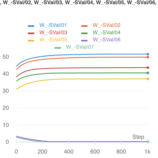 Figure 1: Nuclear Norm minimizer (initialized there) to Ratio Local minimizer.
- Obs: even moving to rank-1, what we can see that the top singular value is dampened, and a collection of small singular vectors/values are able to recreate that loss in the magnitude.
- basically, the problem is, for a given set of entries (I think they can be arbitrary, even though they’re proportional to the true matrix), with a fixed cost for the total norm, but complete freedom with respect to everything else, can you recreate those entries?
- It would be interesting to investigate why our ratio fails: is it a similar kind of failure, where you’re moving some of the mass from the top to the bottom; or, as I expect, it’s going to be a more catastrophic failure, whereby all structure is destroyed, and so it’s basically hopeless to find the truth?
- From Fig. 2, it looks like what happens when the ratio fails, is that you basically start to separate out the singular values. The singular vectors are still roughly right. This suggests something even more elaborate that takes into account variability. Perhaps the spectral norm (max singular value) might do the trick (though this does not admit a computationally-efficient form/gradient).
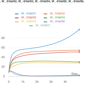 Figure 2: How the ratio penalty fails, with sample size of 1200.
- Obs: trying the noisy version of PGD doesn’t actually do anything.
- feels like it’s not saddle points, so there are actually local minima in the landscape induced by this ratio penalty.
Conclusion
Define \(S^m = \left\{ M : P_{\Omega}(M - M^\star) = 0; \abs{\Omega} = m \right\}\). Then, as you decrease the sample size, \(\abs{\Omega}\), this set grows. For the most part, the nuclear norm min in \(S\) is the truth. But, at some point, this is no longer the case. Let’s actually define an increasing sequences of sets \(\Omega^m\). Then, \(S^m \supset S^{m+1}\). At that point, there is a matrix in \(S^m \setminus S^{m+1}\) with smaller nuclear norm.
From the experiments, it appears that at this boundary condition, this matrix with smaller nuclear norm is very similar to the true matrix. Qualitatively, it seems as if it’s been perturbed, and the singular values dampened, and then noisy singular vectors are introduced to reconstruct the observed entries. Unfortunately, I can’t really think of a principled manner in which to demonstrate this. Perhaps the most fruitful thing here would be to argue in terms of the two norms.
Suppose we’re at the truth (\(M^\star\)). Then perhaps one way to think about what happens is the following: we can always take a step in the direction of the gradient of the nuclear norm from the truth. It just so happens that once your \(S^m\) is sufficiently small, that projection step no longer counteracts the change in norm.
Backlinks
- [[matrix-factorization-to-linear-model]]
- Update: following on from [[experimental-logs-for-matrix-completion]], we have looked at how the nuclear norm fails in the depth-1 case, which is that you dampen the top singular values and reconstruct the residuals from small singular vectors (feels ever so slightly like [[benign-overfitting-in-linear-regression]]).
Matrix Completion Optimization
Let’s try to understand the landscape of optimization in matrix completion.
Matrix Factorization
A celebrated result in this area is (Ge, Lee, and Ma 2016Ge, Rong, Jason D Lee, and Tengyu Ma. 2016. “Matrix completion has no spurious local minimum.” In Advances in Neural Information Processing Systems, 2981–9. University of Southern California, Los Angeles, United States.). They consider the matrix factorization problem (with symmetric matrix, so that it can be written as \(XX^\top\)). Note that this problem is non-convex.1 The general version of this problem, with \(UV^\top\), interestingly, is at least alternatingly (marginally) convex (which is why people do alternating minimization). Under some typical incoherence conditions,2 To ensure that there is enough signal in the matrix, preventing cases where all the entries are zero, say. they are able to show that this optimization problem has no spurious local minima. In other words, for every optima to the function \[ \begin{align*} \widetilde{g}(x) = \norm{ P_\Omega (M - X X^\top) }_F^2, \end{align*} \] it is also a global minima (which means \(=0\)).3 They were inspired, in part, by the empirical observation that random initialization sufficed, even though all the theory required either conditions on the initialization, or some more elaborate procedure.
Proof technique: they compare this sample version \(\widetilde{g}(x)\) to the population version \(g(x) = \norm{ M - X X^\top }_F^2\), and use statistics and concentration equalities to get desired bounds.
Remark. The headline (no spurious minima) sounds amazing, but it’s not actually that non-convex. In any case, as it turns out, it’s basically non-convex (i.e. multiple optima) because you have identifiability issues with orthogonal rotations of the matrix (that cancel in the square). I wonder if the incoherence condition is important here. I don’t think so, as it’s a pretty broad set, so it really does seem like this problem is pretty well-behaved.
A nice thing about the factorization is that zero error basically means you’re done (given some conditions on sample size), since having something that factorizes and gets zero error must be the low-rank answer.To reiterate, they don’t use any explicit penalty (except something that’s helpful for the proof technique to ensure you are within the coherent regime). The matrix factorization form suffices.
Important: something I missed the first time round, but actually makes this somewhat less impressive: they basically assume the rank is given, and then force the matrix to have that dimension. This differs from (Arora et al. 2019Arora, Sanjeev, Nadav Cohen, Wei Hu, and Yuping Luo. 2019. “Implicit Regularization in Deep Matrix Factorization.” arXiv.org, May. http://arxiv.org/abs/1905.13655v3.)’s deep matrix factorization as there they aren’t forcing the dimensions. This doesn’t seem that impressive anymore.
Non-Convex Optimization
src: off-convex.
The general non-convex optimization is an NP-hard problem, to find the global optima. But even ignoring the problem of local vs global, it’s even difficult to differentiate between optima and saddle points.
Saddle points are those where the gradients in the direction of the axis happen to be zero (usually one is max, the other is a min). In the case of gradient descent, since we move in the direction of gradient for each coordinate separately, then we’re basically stuck.
If one has access to second-order information (i.e. the Hessian), then it is easy to distinguish minima from saddle points (the Hessian is PSD for minima). However, it is usually too expensive to calculate the Hessian.
What you might hope is that the saddle points in the problem are somewhat well-behaved: there exists (at least) one direction such that the gradient is pretty steep. This way, if you can perturb your gradient, then hopefully you’ll accidentally end up in that direction that lets you escape it.
That’s where noisy gradient descent (NGD) comes into play. This is actually a little different to stochastic gradient descent, which is noisy, but that noise is a function of the data. What we want is actually to perturb the gradient itself, so you just add a noise vector with mean 0. This allows the algorithm to effectively explore all directions.4 In subsequent work, it has been established that gradient descent can still escape saddle points, but asymptotically, and take exponential time. On the other hand, NGD can solve it in polynomial time.
What they show is that NGD is able to escape those saddle points, as they eventually find that escape direction. However, the addition of the noise might have problems with actual minima, since it might perturb the updates sufficiently to push it out of the minima. Thankfully, they show that this isn’t the case. Intuitively, this feels like it shouldn’t be that hard – if you imagine a marble on these surfaces, then it feels like it should be pretty easy to perturb oneself to escape the saddles, while it seems fairly difficult to get out of those wells.
Proof technique: replace \(f\) by its second-order taylor expansion \(\hat{f}\) around \(x\), allowing you to work with the Hessian directly. Show that function value drops with NGD, and then show that things don’t change if you go back to \(f\). In order for this to hold, you need the Hessian to be sufficiently smooth; known as the Lipschitz Hessian condition.
It turns out that it is relatively straightforward to extend this to a constrained optimization problem (since you can just write the Lagrangian form which becomes unconstrained). Then you need to consider the tangent and normal space of this constrain set. The algorithm is basically projected noisy gradient descent (simply project onto the constraint set after each gradient update).
The Form of the Loss in Matrix Completion
Key: everything goes through the loss function!
What’s wacky is that, usually when we think of neural networks, we have some data pairs \((x,y)\), and the usual operation is that you feed your input \(x\) into your network, and out pops your prediction of \(y\). Another way to put that is, you assume that \(y = f(x)\) for some unknown function \(f\), and the goal of training a neural network is to emulate that unknown \(f\).
In particular, if you ignore the non-linear components, and we deal with a fully connected neural network, then what it boils down to is repeatedly hitting the input vector \(x\) with weight matrices \(W_1, W_2, \ldots, W_N\).
Everything gets turned on its head, it feels, when you consider the problem of Matrix Completion. The architecture is exactly the same, except now the \(x\)’s have disappeared, and what you’re left with are just the weight matrices, and the way you use them is all through this new loss function:
\[ \begin{align*} \norm{ P_{\Omega}(\hat{W}) - P_{\Omega}(W) }_{2}^2, \end{align*} \]
where the \(P_{\Omega}\) is the vectorized form of the relevant entries shown in \(W\), and the \(\hat{W}\) is precisely the product of all the individual weight matrices (since it’s linear it’s equivalent to hitting \(x\) with one matrix). Thus, there’s not really a nice one-to-one in terms of what \((x,y)\) are here. But those are ultimately superfluous.
Really, everything can be derived through the loss function. That is, the normal loss function looks like:
\[ \begin{align*} \sum_{i} L(y_i, f(x_i)). \end{align*} \]
The diagrams we build to describe our networks can sometimes be misleading.
Backlinks
- [[extending-the-penalty]]
- currently, in the case of matrix completion, the penalty is straightforward, since we have a product matrix already as our final goal [[the-form-of-the-loss-in-matrix-completion]].
Effectiveness of Normalized Quantities
In the context of matrix completion, it is known that the nuclear norm, being a convex relaxation of the rank,1 You can think of these as the matrix version of the \(l_1\) to \(l_0\) duality. has very nice low-rank recovery properties. However, in sparser regimes (not enough observed entries), the nuclear norm starts to falter. This is because there is sufficient ambiguity (equivalently, not enough constraints on the convex program).2 Recall that the convex program is something like \(\min \norm{W}_{\star} \text{ s.t. } P_{\Omega}(W^\star) = P_{\Omega}(W)\), where the \(P_{\Omega}\) is the convenient operator to extract the observed entries Thus, minimizing the nuclear norm doesn’t actually recover the true matrix.
However, it turns out that simply normalizing it works wonders. Consider the penalty, \(L_{\star/F}\), which is given by
\[ \begin{align*} \frac{L_1}{L_2} = \frac{ \sum \sigma_i }{ \sqrt{ \sum \sigma_i^2 } }, \end{align*} \]
where \(\sigma_i\) are the singular values. The idea here is that we’re interested in the relative size of our singular values, not the absolute sizes. Using the nuclear norm as a penalty means that you can simply push down all the entries of your matrix to.
Compare this to the gradient accelerator ADAM, which, in a nutshell considers a normalized gradient sequence. That is, the update step is given by3 Granted, I am hiding some details, like how the summation is actually weighted to prioritize the most recent gradient, the division is element-wise, plus some computation tricks to ensure no division by zero.
\[ \begin{align*} \frac{ \sum g_t }{\sqrt{\sum g_t^2}}, \end{align*} \]
Remark. Experiments show that it is the denominator that is more important than the numerator. So, really, what seems to be important is that you’re normalizing each gradient parameter by the magnitude of the gradient. I feel like there’s something statistical about all this that we might be able to learn.
I tried to do something about the Hadamard product, but my feeling is that this cannot be captured through matrix operations alone.where \(g_t\) is the gradients of the loss. The reason I bring up these two quantities is that it turns out that only by using these two methods do we get something interesting coming out. It could very well be coincidence that they have a similar form, but I suspect that perhaps normalized quantities are somehow superior in the deep learning regime.
Parallels
Originally I thought this felt a lot like our scores in #statistics, but upon further inspection I realized that this would only hold if you have assume zero mean, since the entries aren’t actually centered (and no \(\sqrt{n}\)). The problem there is that all the singular values are positive, so it seems sort of weird to say that this is essentially a \(Z\)-score of the null hypothesis that these were drawn from a zero-mean normal distribution.
Backlinks
- [[project-penalty]]
- As it turns out, there is an explicit penalty. And it’s given by the ratio of the nuclear norm and the Frobenius norm (see [[effectiveness-of-normalized-quantities]]).
- [[exponential-learning-rates]]
- Two key properties of SOTA nets: normalization of parameters within layers (Batch Norm); and weight decay (i.e \(l_2\) regularizer). For some reason I never thought of BN as falling in the category of normalizations, ala [[effectiveness-of-normalized-quantities]].
- [[fractals]] Scale-free, or scale-invariance. If you’re given a picture of some rock, then you can’t tell what scale it is at, since you have self-similarity across scaling. Hence you need that reference scale on the bottom right. I wonder if this relates to scale-invariance (à la [[effectiveness-of-normalized-quantities]]).