#networks
Testing a PA model
Testing Problem
We are interested in the following testing problem: how do we distinguish between a graph generated from a PA model, and a graph from a configuration model with the same degree distribution as the first graph?
The point of this test is, in part, to determine what are the defining properties of a PA model besides the fact that it is scale-free. Of course, we consider the undirected version, as otherwise it would be trivial (since PA vertices all have an out-degree of \(m\)).
Our first idea was to take inspiration from (Bubeck, Devroye, and Lugosi 2014Bubeck, Sébastien, Luc Devroye, and Gábor Lugosi. 2014. “Finding Adam in random growing trees.” arXiv.org, November. http://arxiv.org/abs/1411.3317v1.), and consider centroids1 defined as the vertex whose removal results in the minimum largest component. However, given the lack of an off-the-shelf implementation of this algorithm in R, we decided to look for a simpler test. As it turns out, if we just look at the nodes with the highest degree (together), we get interesting results.
set.seed(5)
library(igraph)
# create induced subgraph by taking the k largest degree nodes
create_induced_topk <- function(g, k) {
  n <- gorder(g)
  dg <- degree(g)
  induced_subgraph(g, order(dg)[(n-k+1):n])
}
# compares to graphs g,h to test which is which
tester <- function(g, h, k=20) {
  g2 <- create_induced_topk(g, k)
  h2 <- create_induced_topk(h, k)
  # if sizes are the same, we should return 1/2
  ifelse(gsize(g2) == gsize(h2), .5, gsize(g2) < gsize(h2))
}
Consider the following test: for a graph \(G\), calculate the induced subgraph by taking the top-\(k\) degree vertices. Which model produces an induced subgraph with more edges?
n <- 100
k <- 5
g <- sample_pa(n, power=1, m=2)
(g2 <- create_induced_topk(g, k))
## IGRAPH 99eb979 D--- 5 7 -- Barabasi graph
## + attr: name (g/c), power (g/n), m (g/n), zero.appeal (g/n), algorithm
## | (g/c)
## + edges from 99eb979:
## [1] 2->1 3->1 3->2 4->1 4->3 5->1 5->4h <- sample_degseq(degree(g), method="vl")
(h2 <- create_induced_topk(h, k))## IGRAPH bdfa659 U--- 5 6 -- Degree sequence random graph
## + attr: name (g/c), method (g/c)
## + edges from bdfa659:
## [1] 1--2 3--4 1--5 2--5 3--5 4--5par(mfrow=c(1,2))
Plot(g2)
Plot(h2)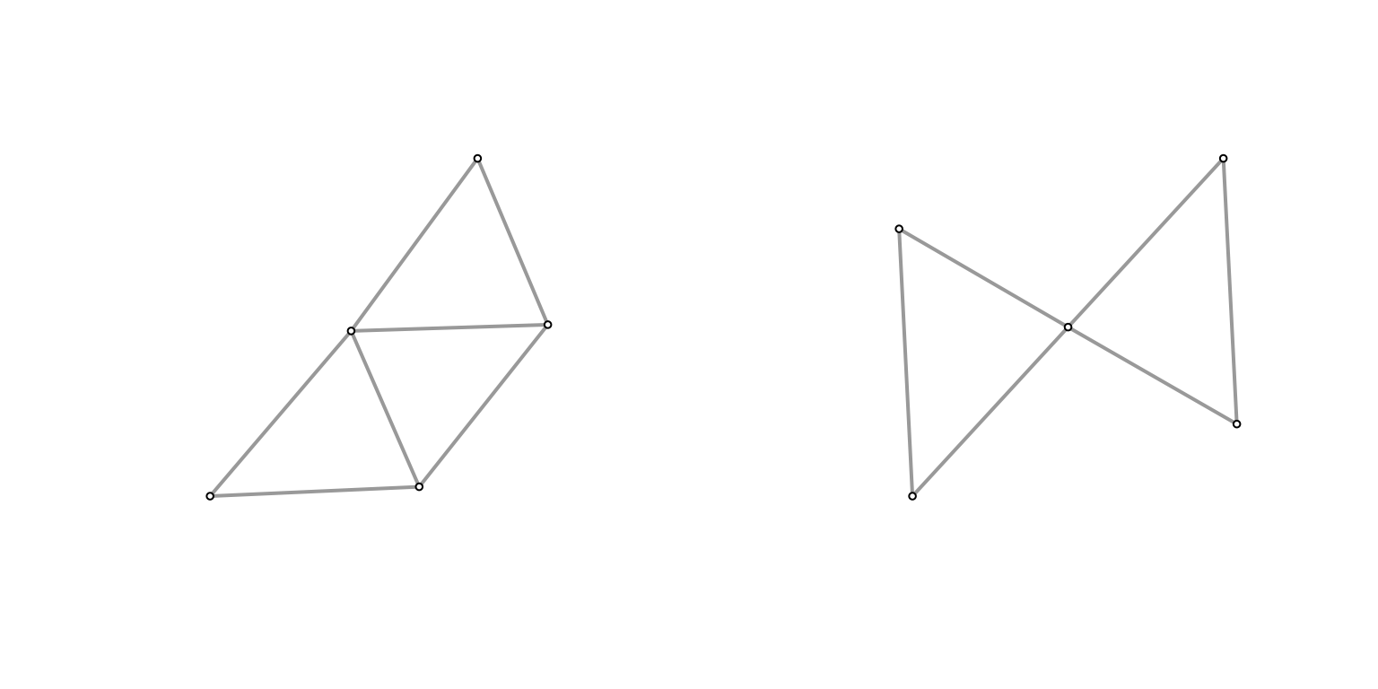
They don’t look that different at \((n,k) = (100,5)\), and the size of the graph is similar (edge count). What if we turn it up a notch?
n <- 1000
k <- 10
g <- sample_pa(n, power=1, m=2)
(g2 <- create_induced_topk(g, k))
## IGRAPH fdeb1f2 D--- 10 13 -- Barabasi graph
## + attr: name (g/c), power (g/n), m (g/n), zero.appeal (g/n), algorithm
## | (g/c)
## + edges from fdeb1f2:
## [1] 2->1 3->1 3->2 4->1 4->3 5->1 6->2 7->4 7->6 8->1 9->3 9->6
## [13] 10->3h <- sample_degseq(degree(g), method="vl")
(h2 <- create_induced_topk(h, k))## IGRAPH 1468645 U--- 10 22 -- Degree sequence random graph
## + attr: name (g/c), method (g/c)
## + edges from 1468645:
## [1] 1-- 3 2-- 3 1-- 4 2-- 4 3-- 4 1-- 5 2-- 5 1-- 6 2-- 6 4-- 6 3-- 7 4-- 7
## [13] 1-- 8 3-- 8 6-- 8 7-- 8 1-- 9 3-- 9 1--10 3--10 4--10 5--10par(mfrow=c(1,2))
Plot(g2)
Plot(h2)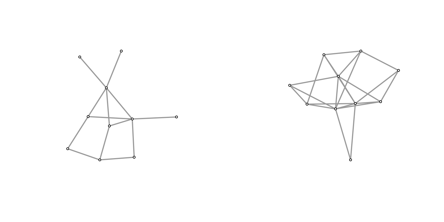
It feels like the induced subgraph from the configuration model is more densely connected (closer to a clique). Why might this be? In the case of the configuration model, if you consider the top \(k\) degree’d vertices, then there’s a very high probability of them being connected to one another2 if we take the half-edge formulation, then for any half-edge, it’s more likely to be connected to those with higher degrees (since they possess more half-edges). but they themselves have more half-edges, so it should amount to more edges between them.. Meanwhile, for a PA model, roughly we have that high degree nodes are older/earlier, and so probably have a slightly larger chance of connecting to each other than, say, a younger and an older node (since early on there aren’t many other options), but this is probably a much smaller effect.
To test this, let’s run some simulations. Here, I’ve run all combinations of \(n \in [100, 500, 1000]\) and \(k \in [5, 10, 15]\).
nsim <- 1000
ns <- c(100, 500, 1000)
ks <- c(5, 10, 20)
df <- expand.grid(k=ks, n=ns)
df$prob <- 0
cnt <- 1
for (k in ks) {
  for (n in ns) {
    res <- c()
    for (i in 1:nsim) {
      # generate graph
      g <- sample_pa(n, power=1, m=2)
      # generate the equivalent configuration model
      h <- sample_degseq(degree(g), method="vl")
      res <- c(res, tester(g, h, k=k))
    }
    df$prob[cnt] <- mean(res)
    cnt <- cnt + 1
  }
}
knitr::kable(df)| k | n | prob |
|---|---|---|
| 5 | 100 | 0.7475 |
| 10 | 100 | 0.8180 |
| 20 | 100 | 0.8705 |
| 5 | 500 | 0.9740 |
| 10 | 500 | 0.9940 |
| 20 | 500 | 0.9980 |
| 5 | 1000 | 0.9990 |
| 10 | 1000 | 1.0000 |
| 20 | 1000 | 1.0000 |
Clearly, we see a positive relationship between both \(k\) and \(n\) with respect to testing accuracy. Though, at \(n=1000\), it’s essentially as good as it’s going to get.
“Theory”
Here’s some hand-wavy calculations. For the simplest case of \(k=2\), we are interested in the probability that the top two degree vertices are connected. Let \(d_1, d_2\) be these degrees (and the respective vertex too). For the configuration model, for any given half-edge of \(d_1\), the probability that it’ll be connected to \(d_2\) is given by \(\dfrac{d_2}{D - d_1}\). Then, the probability that they’re connected is given, roughly, by \(\dfrac{d_1 \cdot d_2}{D}\).
Now consider the preferential attachment model. For now, let’s assume that \(d_1\) arrived before \(d_2\).3 can’t really WLOG here, but it feels close enough In other words, what we’re interested is the probability that one of the \(m\) vertices chosen by \(d_2\) was \(d_1\). Denote the arrival time4 which also corresponds to the number of vertices at that time of these two vertices as \(t_1\) and \(t_2\), respectively. Then, the probability is given by \(\dfrac{d_1(t_2)}{m \cdot t_2}\). The further out the \(t_2\), the larger the denominator, but also the more time \(d_1\) has had to amass its popularity.
The key is that it’s independent of \(d_2\) (i.e. the degree of the second vertex) – it would be the same probability for any other node at time \(t_2\).
Dynamic Graph Models
The traditional way of thinking about networks is to treat them as essentially fixed, and samples from some generative model. Of course, we all know that networks don’t just spontaneously appear. That being said, a) collecting the entire history of a network’s evolution to its current state is often impossible, and b) dynamic models introduce too many more degrees of modelling freedom, so the purists generally shy away from it.
A useful dynamic model is one where the dynamics is fairly simple, and yet interesting global features still manifest themselves (in the spirit of [[complexity-theory]]). The classic example of this is the Preferential Attachment (PA) model, which, by a very simple rich-get-richer adjustment to the Uniform Attachment (UA) model creates a power-law degree distribution. A simple description of these models is, at each time step \(t\), we introduce a new vertex \(v_t\), and we add \(m\) new edges from this new one.1 i.e. each vertex has out-degree \(m\). The probability that an existing vertex has an edge to this vertex is either uniform (UA), or weighted by its current degree (PA),
\[ \begin{align*} P(A_{v_t, v_i}) = \frac{d_i}{\sum d_i}, \quad \forall i \in E. \end{align*} \]
Thanks to Bubeck, a completely different view of PA models is to focus on the temporal/growth aspect of it – by their very dynamics, we unlock a slew of different questions to ask. At a high level, the questions revolve around how much temporal information is recoverable from the final state?
For instance, we might be interested in determining the “seed” of a network2 You can adjust the model by starting with a fixed seed network (instead of a single node)., e.g. to figure out the early core of the internet. In the case of a pandemic, reverse-engineering the infection/contact network might give insight into the early actors. Of course, no real-life network follows a PA model exactly, which leads to the more practical question of, how much temporal information is recoverable even under a corrupted model?
A simple corruption is to simply inject random edges (sort of like having an ER graph embedded in the graph) – the opposite being having missing data (or both!). There’s probably an asymmetry here: adding edges makes retrieval more difficult than deleting edges. A simple extreme example: in the PA model with \(m=1\), the resulting graph is always a tree, which remains true when deleting but not when adding at random. Thus, any algorithm that relies on the tree breaks down.
Existing Work
The first problem (via this blog-post) involves asking questions about the seed graph (or the root). In a nutshell, the centroid of a tree, which is defined as the vertex whose removal results in the minimum largest component, is actually a good estimate of the root. Proving such a statement utilizes the probabilist’s favorite home appliance, the Polya Urn.
 Figure 1: The Centroid (1)
A similar problem (older blog-post) looks at the question of whether or not the seed graph has any influence (in the limit). Formally, we consider if the total variation distance between the two limiting distributions of two different seeds is bounded away from zero. This is a weaker requirement, since being able to recover the seed implies it has influence.
This line of inquiry can also be framed as follows: if we think about social networks, then what you might be interested in is this notion of the early-bird advantage – just by being there early, you get outsized returns (degree). Suppose people enter a network with the object of maximizing that return. Then it almost becomes something like a multilevel marketing (pyramid) scheme.
Open Problems
- Our intuition tells us that the network effect is definitely something that advantages people who are earlier to a platform. In a very similar vein to the rich-get-richer scheme, being early is essentially synonymous with being rich. However, it needn’t be that way. I think it might be useful to try to come up with a model that is essentially arrival-time agnostic, i.e. you have exchangeability at the node-level, which is something you generally get for free when you’re doing generative static network models, but is explicitly unavailable for dynamic models. Having such a model might help us elucidate the structural differences between two scale-free, dynamic models that differ on that one point.
Grand Theory of Social Networks
Anyone who knows me would be unsurprised that I have a grand theory for social networks (hence the title). In fact, this idea has been at the back of my head for many years (like with the dozen other things on the backburner), but a recent AI #podcast episode inspired me to see if there’s something to it. In fact, in 2016, I wrote some initial thoughts down, part of which I will reproduce below.
The generative models for social networks of yesteryear were these beautifully crafted simple models that yielded complex epiphenomena at scale. Small worlds/random ties produce small diameter; preferential attachment yields power law degree distributions. Are there other such simple ideas that can produce the complex dynamics of social network formation?
My hope is that homophily, together with the randomness of human personality/traits, might be the driving force of the social network realizations. Actually, I think it is the combination of having characteristics, and the relative ranking/disposition towards certain characteristics, that drives the global complexity of network. Thus, this dream falls in the realm of complexity theory.
Homophily
Let us model individuals as high-dimensional random vectors \(\in \mathbb{R}^{p}\) that correspond to different characteristics. The dimension of the ambient space, \(p\), shall vary, as it might be the case that the magnitude of \(p\) drives some of the emergent properties.1 For instance, one could claim that as civilization progresses, you have more characteristics to compare, which might then explain differences between rural and modern social networks. Similarly, the choice of the noise distribution (standard vs fat-tailed) might also have implications – for now, we default to Gaussian noise.
The basic idea is that relationships are formed based on similarity (vectors/individuals that are close in some metric should be friends). This idea is clearly not new – objects such as \(k\)-nearest neighbour graphs or the \(\epsilon\)-neighbour graph have been proposed and studied extensively. However, it seems they’re mainly used to generate ad-hoc similarity graphs, which is far removed from a social network.
The piece of insight from the podcast episode – and why I am revisiting this idea many years down the road – is that homophily on its own doesn’t really produce sufficiently complex graphs.2 What do I mean by this? Clearly (?) for any graph \(G\) there exists a set of vectors such that its similarity graph
set.seed(0)
n <- 5 # no. of people
p <- 10 # no. of characteristics
X <- matrix(rnorm(n*p), nrow=n)
Noisy Networks
src: Chang, Kolaczyk, and Yao (2018Chang, Jinyuan, Eric D Kolaczyk, and Qiwei Yao. 2018. “Estimation of subgraph density in noisy networks.” arXiv.org, March. http://arxiv.org/abs/1803.02488v3.), Li, Sussman, and Kolaczyk (2020Li, Wenrui, Daniel L Sussman, and Eric D Kolaczyk. 2020. “Estimation of the Epidemic Branching Factor in Noisy Contact Networks,” February. http://arxiv.org/abs/2002.05763.)
A common task in network analysis is to calculate a network statistic, from which some conclusion can be gleaned. Oftentimes you’ll have a table of typical summary statistics for your graphs, and they can be either (average) node-level statistics (like centrality), or global statistics (like edge density). There is usually not much import to those tables – mainly used just so people can get a feel for the graph/dataset.
Sometimes though you’re interested in some particular real-valued functional of the network. For instance, in my previous work, we were interested in unbalanced triangles. Another statistic, very relevant to #coronavirus, is the branching factor, or \(R_0\), of a contact network (see Li, Sussman, and Kolaczyk (2020Li, Wenrui, Daniel L Sussman, and Eric D Kolaczyk. 2020. “Estimation of the Epidemic Branching Factor in Noisy Contact Networks,” February. http://arxiv.org/abs/2002.05763.) for more details).
Whenever you have a statistic, you might want to know two things: how confident are you of this value, or what is the “variability” of this statistic; and whether or not this statistic is significant. Let’s take this latter approach first. The idea here is that we have some hypothesis that we want to test, and so we need to first construct a null hypothesis, and the statistic is the mechanism (or measure) through which which we can judge the significance of our test. In the former case, all that we really want is just a set of confidence intervals for our statistic. It’s almost the same thing, except there is no hypothesis – all that is required is a random model that lets you define the form of the noise, and therefore construct confidence intervals.
So in fact, there is a subtle difference between these two things. For the most part, I have been thinking about the latter (hypothesis testing), but attaching confidence bands to point estimates in networks is also an interesting research question.
Noise Model
The noise model analyzed in these papers is very straightforward. It essentially follows the paradigmatic signal + noise model in statistics. Fix a graph \(G\) (defined by its adjacency matrix \(A\)), which we think of as the ground truth. Then the noisy observation (adjacency matrix \(\widetilde{A}\)) are produced by random bit-flips (0 to 1 or 1 to 0). For simplicity, the random bit-flips are modelled with only two parameters: \(\alpha\), the Type-1 error, and \(\beta\), the Type-2 error. That is,
\[ \begin{align*} P(\widetilde{A}_{ij} = 1 \given A_{ij} = 0) = \alpha, \quad P(\widetilde{A}_{ij} = 0 \given A_{ij} = 1) = \beta, \end{align*} \]
Thus, you’ve reduced the whole problem to estimating two parameters.1 Which feels a little extreme. Unsurprisingly, you use #method_of_moments to estimate them. However, because you have two parameters, you’re going to need more than one sample (i.e. two).
Actually, I think it’s a little more complicated than that (it’s not really a degree-of-freedom thing). One might think that with a large enough graph, you can probably split in two, and estimate the parameters on each half (and they’d be independent). However, I suspect the problem is that the model is a little too general, so if your \(\alpha, \beta\) are too large, then you can’t really guess anything.2 i.e. you have no control of what’s signal and what’s noise. My guess is that if you have two samples, then you have access to the intersection/set-difference, which makes it more feasible to estimate things. But the thing is that this then relies on the intersection.
This makes me think that a) if you restrict the \(\alpha, \beta\) to be suitably small, then you can probably be okay with one sample; and b) this model is actually pretty restrictive.3 I mean, in terms of the space of possible samples it is fine, but I guess like any model, you really don’t want your results to depend so much on the assumptions.
This is similar to the #stochastic_blockmodel, in that these parameters are really just nuisance parameters. In that model, you can actually estimate many things without actually knowing these nuisance parameters.
Remark. It might seem weird to fix a graph. Clearly I cannot be too against this notion, since the test I propose also assumes a fixed graph. However, in that particular setting, I felt that was the best option. Not something that I thought was particularly realistic (but the alternatives, considering parametric models seemed even more riddled with problems).
In my opinion, this particular model must be considered together with the particular application. A concrete example would be protein networks. I don’t know how these datasets are generated, and so it is unclear to me if such a noise model would be an accurate representation. The key thing here is that this is how we’re modelling the multiple draws/samples.A Better Model?
Two things come to mind. First is model-fitting and checking, though not necessarily singularly focused on this particular noise model. As I’ve said before, almost all network models are a terrible model for real-life data, especially the parametric ones. This particular model is technically parametric, but very different. So what we want are diagnostic checks to see how comformal our data is to the models. Since this procedure utilizes the fact that you have multiple samples, then that also means that you probably should be able to use that for diagnostics.
Along a similar line, it seems that what we would want is a more robust version of this noise model. Or, another way to think about this is that, what you want are estimators that are more robust to the model assumptions.4 like median for measure of centrality not assuming normality in the errors. I’m not really sure what the form of this would be: something a little more non-parametric?
If we are interested in the application of contact networks, then it might be fruitful to consider in isolation, and come up with a particular noise model that we think suits this dataset.5 and potentially the paper could be a general type of paper that we can then demonstrate specializing to different data types.
Dyadic Imbalance in Networks
src: link
- Actually does Local Testing on Graphs, as I’ve wanted to do. But in a very simple manner. Basically, you define dyadic imbalance as the fraction of cycles that are unbalanced. Cool.
- they also basically handle multiplex networks by essentially merging everything into one graph. Cool.
- data
- what is sort of interesting is their application to IR is quite extensive (and very different to the social network setting)
- they also have something related to voting decisions in the US Congress, which seems pretty interesting (like Wikipedia admin voting)
- method
- they use the permutation test (which they explain in a very roundabout way)
- they use something called a Heckman Selection Model, which I highly doubt solves the problem, but maybe it does?
- this is some model that claims to fix sample selection biases
- basically, they treat it like a covariate. but this is where we might be able to show something bad about their model. Basically, just like the whole spurious test when running linear regression on time series, doing node covariate regression, especially when you have graph statistics that are highly dependent is going to screw you over
Nonparametric Testing on Graphs
Lit Review
- Testing Equivalence of Clustering, (Gao and Ma 2019Gao, Chao, and Zongming Ma. 2019. “Testing Equivalence of Clustering.” arXiv.org, October. http://arxiv.org/abs/1910.12797v2.)
- abstract
- “In this paper, we test whether two datasets share a common clustering structure. As a leading example, we focus on comparing clustering structures in two independent random samples from two mixtures of multivariate Gaussian distributions. Mean parameters of these Gaussian distributions are treated as potentially unknown nuisance parameters and are allowed to differ. Assuming knowledge of mean parameters, we first determine the phase diagram of the testing problem over the entire range of signal-to-noise ratios by providing both lower bounds and tests that achieve them. When nuisance parameters are unknown, we propose tests that achieve the detection boundary adaptively as long as ambient dimensions of the datasets grow at a sub-linear rate with the sample size.”
- abstract
- Minimax Rates in Network Analysis: Graphon Estimation, Community Detection and Hypothesis Testing, (Gao and Ma 2018Gao, Chao, and Zongming Ma. 2018. “Minimax Rates in Network Analysis: Graphon Estimation, Community Detection and Hypothesis Testing.” arXiv.org, November. http://arxiv.org/abs/1811.06055v2.)
- tests involving ER vs SBM
- more general test that handle “degree-corrected” i’m guessing (via his paper with Lafferty)
- results in a nice test that involves counts of subgraphs/motifs (essentially boiling down to edges, vees and triangles)
- it’s independent of the heterogeneity of the degree distribution, so you don’t have to estimate those nuisance parameters
- Network Global Testing by Counting Graphlets (Jin, Ke, and Luo 2018Jin, Jiashun, Zheng Tracy Ke, and Shengming Luo. 2018. “Network Global Testing by Counting Graphlets.” arXiv.org, July. http://arxiv.org/abs/1807.08440v1.)
- reminds me of the method-of-moments type thing we did in the [[parameter-estimation-in-sbm]] paper
Backlinks
- [[master-paper-list]]
- [[nonparametric-testing-on-graphs]] (this could also be a more applied paper, that discusses the general problem with doing tests, or just modeling things in social networks)
- JASA
- [[nonparametric-testing-on-graphs]] (this could also be a more applied paper, that discusses the general problem with doing tests, or just modeling things in social networks)
Honduras Face Project
Given a signed social network, various demographics, and faces, what interesting questions can be answered?
Existing Literature
- The Faces of Group Members Share Physical Resemblance (doi):
- similar-looking people are more likely to be friends
- not particularly surprising. the main question is one of causal direction?
- Multidimensional Homophily in Friendship Networks (link):
- this paper doesn’t actually seem that interesting. not sure what linear model they’re using, but ignoring that, what they show is that the coefficient for two variables (same sex, same ethnicity) are positive while the interaction of these two variables is negative.
- but (I’m pretty sure) all that tells you is that it’s not an additive relationship, so you get diminishing returns for homophily.
- this seems very plausible (they do mention this in the discussion). there’s redundancies involved.
- Attractiveness and Symmetry: much existing work showing that people rate averageness as more attractive
- i.e. deviation from the norm is penalized.1 except when dealing with high fashion models, where singularity is prized. this was mentioned in a recent episode on Tyler’s podcast
Backlinks
- [[master-paper-list]]
- [[honduras-face-project]]
- Nature
- [[honduras-face-project]]
- [[pediatric-transfer-learning]]
- I guess this isn’t particular to pediatric research; anytime you have some more common/majority group of individuals, and you want to study an under-represented group (or, the more stupid thing would be to think that the models trained on the majority group are somehow universal, but in fact fail completely when trained on a minority: a problem I came across in the [[honduras-face-project]]).
New Balance Theory
Balance Theory as it stands is a fairly straightforward and well-established idea from sociology about how signed graphs should form. Most people assume that it is basically an asymptotic realization (with enough time, all graphs will end up being exactly balanced). But actually wouldn’t it be great if we could show that the negative ties actually have some value.
Let’s start with what we know about balance. A graph is weakly balanced if and only if it can be decomposed into disjoint communities. Another way to characterize this is that it becomes perfectly polarized. So one way to think about moving away from balance is actually protecting our society from extreme polarization.
It’s sort of similar to the notion of weak links being these important connections that facilitate communication between disparate groups. This basically takes the more extreme form, no longer just about communication and understanding between groups, but more importantly, controlling animosity.
So in some sense, animosity is always going to be inevitable. However, if you have animosity, and you have strong inclinations for balance, you’re going to end up in a polarized world. So what you want actually are the mediators that are able to prevent the network degenerating into factions.
Though, and I think this is something crucial about all these models that is underappreciated: we have various scales to consider (hierarchical modelling), as we as various dimensions through which we can differentiate ourselves. It seems that the multi-faceted nature of our lives should give rise to interesting complex phenomenon.
Concrete Plan
One idea is to see if we can model how things play out on social media like Twitter. Can we actually identify these mediators and show that given enough of them, and if they have enough clout, then they can stop the collapse of social networks?
Another idea takes a more generative model approach. Balance, for one thing, is a global property, so the question is what kinds of local behaviour can produce the kinds of structure that we see in the real world.
Backlinks
- [[master-paper-list]]
- “Bridgers” in Unbalanced Triangles: [[new-balance-theory]]
- Nature
- “Bridgers” in Unbalanced Triangles: [[new-balance-theory]]
AB Testing in Networks
source: h.
Summary
- Typical A/B testing (RCT) is done uniformly across the whole population.
- the resolution of the \(t\)-statistic across treatment and control assumes that the TE is independent of treatment
- this assumption is usually treated as given, but difficulties when subjects can interact
- example: group effect, if enough of your friends have the treatment, then you’ll respond positively
- when you have (social) networks, or just people interacting on the same system, what to do?
- expand your unit of experiment: instead of subject, just find components in your graph. to be explicit, this simply means assigning the same treatment to all those in that component.
- however, in most social network settings, we have a very large component (and you get small diameter for free)
- then you’re basically stuck. you could partition into subgroups, but there will always be edges between groups
- could turn into a graph cut problem, aka community detection problem, where you’re finding a partition that minimizes connecting edges.
- in certain settings, the networks are collections of small components. then you’re good to go.
- however, in most social network settings, we have a very large component (and you get small diameter for free)
- my feeling/intuition is that academics will try to measure this network effect. getting into #causal_inference territory.
- oftentimes, this is done post-hoc, so rerunning the experiment is not possible.
- expand your unit of experiment: instead of subject, just find components in your graph. to be explicit, this simply means assigning the same treatment to all those in that component.
- so, if you widen your unit, you’re going to lose power
- fewer experimental units
- differences in units (large vs small, different behaviours)
- it’s like the propensity matching problem, you want similar units, so it’s easier to extract the treatment effect
- solution, part (a): do matching, but in a stratified way
- solution, part (b): expand your model
- the usual model is \(y_i \sim \mu + \tau t_i\), where \(t_i\) is indicator function of treatment, and \(\tau\) is our (average) treatment effect.
- because we have these mini-units, we can do some further modelling here, so that our response is not just a function of the treatment \(t_i\), but also a function of the groups within this unit.
- spill-over effects:
- \(y_i \sim \mu + \tau t_i + \gamma a_i \cdot T\), where \(a_i\) is the column of the adjacency matrix, and \(T\) is the vector of treatments, so \(a_i \cdot T\) is just a cute way to count the number of neighbors
- since by definition, a neighbour must be in the same treatment, you can just replace \(T\) with the ones vector.
- this is a first-order spill-over effect, and it seems like it is simply additive.
Highlights
One particular area involves experiments in marketplaces or social networks where users (or randomized samples) are connected and treatment assignment of one user may influence another user’s behavior.
Typical A/B experiments assume that the response or behavior of an individual sample depends only on its own assignment to a treatment group. This is known as the Stable Unit Treatment Value Assumption (SUTVA). However, this assumption no longer holds when samples interact with each other, such as in a network. An example of this is when the effects of exposed users can spill over to their peers.
Experiments in social networks must care about “spillover” or influence effects from peers.
we lose experimental power. This comes from two factors: fewer experimental units, and greater inherent difference across experimental units.
cluster samples into more homogeneous strata and sample proportionately from each stratum.
Another aspect of concern is that treatment can in theory affect not just experiment metrics but also the graph topology itself. Thus graph evolution events also need to be tracked over the course of the experiment.