#proj:interpolation

src: (⊕Bubeck and Sellke 2021Bubeck, Sébastien, and Mark Sellke. 2021. “A Universal Law of Robustness via Isoperimetry.” arXiv.org, May. http://arxiv.org/abs/2105.12806v1.)

Here’s another attempt to explain the overparameterization enigma found in deep learning (\(p >> n\)).

• to fit (interpolate) \(n\) data points of \(d\) dimensions, one requires \(nd\) parameters if one wants a smooth function (without the smoothness, \(n\) should suffice)
• thus, the overparameterization is necessary to ensure smoothness (which implies robustness)

Their theorem/proof works in the contrapositive: for any function class smoothly parameterized by \(p\) parameters (each of size at most \(\text{poly}(n,d)\)), and any \(d\)-dimensional data distribution satisfying mild regularity conditions, then any function in this class that fits the data below the noise level must have Lipschitz constant larger than \(\sqrt{\dfrac{nd}{p}}\).

• note that this result doesn’t say that you’ll fit a smooth function if you’re overparameterizing – just that if you don’t have enough parameters, then there’s no way you’re fitting a smooth one.
  • thus, in the context of scale (à la [[gpt3]]), this result says that scale is necessary to achieve robustness (though not sufficient).
• the noise level here is defined as the expected conditional variance \(\sigma^2 := \E[\mu]{\text{Var}(y \given x)} > 0\). noise is necessary from a theoretical perspective, as it prevents fitting a smooth classifier with perfect accuracy.

src: (Feldman ⊕2019Feldman, Vitaly. 2019. “Does Learning Require Memorization? A Short Tale about a Long Tail.” arXiv.org, June. http://arxiv.org/abs/1906.05271v3.)

A different take on the interpolation/memorization conundrum.

The key empirical fact that this paper rests on is this notion of data’s long-tail.11 This was all the rage back in the day, with books written about it. Though that was more about #economics and how the internet was making it possible for things in the long tail to survive. Formally, we can break a class down into subpopulations (say species22 Though they don’t have to be some explicit human-defined category.), corresponding to a mixture distribution with decaying coefficients. The point is that this distribution follows a #power_law distribution.

Now consider a sample from this distribution (which will be our training data). You essentially have three regimes:

1. Popular: there’s a lot of data here, you don’t need to memorize, as you can take advantage of the law of large numbers.
2. Extreme Outliers: this is where the actual population itself is already incredibly rare, so it doesn’t really matter if you get these right, since these are so uncommon.
3. Middle ground: this is middle ground, where you still might only get one sample from this subpopulation, but it’s just common enough (and there are enough of them) that you want to be right. And since they’re uncommon, you basically only have one copy anyway, so your best choice is to memorize.

Key: a priori you don’t know if your samples are from the outlier, or from the middle ground. So you might as well just memorize.33 What you have is that actually, what you don’t mind is selective memorization. Though it’s probably too much work to have two regimes, so just memorize everything.

My general feeling is that there is probably something here, but it feels a little too on the nose. It basically reduces the power of deep learning to learning subclasses well, when I think it’s more about the amalgum of the whole thing.

src: (Bartlett et al. ⊕2020Bartlett, Peter L, Philip M Long, Gábor Lugosi, and Alexander Tsigler. 2020. “Benign overfitting in linear regression.” Proceedings of the National Academy of Sciences of the United States of America vol. 80 (April): 201907378.).

• references:
  • slides, better exposition
  • new paper that generalizes this: “Benign overfitting in the large deviation regime”, via arXiv
• setting:
  • linear regression (quadratic loss), linear prediction rule
    • important: we are actually thinking about the ML regime, whereby there isn’t just a true parameter, but that there is a best one by considering the expectation (which, under general settings, corresponds to what would be the “truth”).
    • important: they are considering random covariates in their analysis! I guess this is pretty standard practice, when you’re calculating things like risk
    • that is, you can think of linear regression as a linear approximation to \(\mathbb{E} ( Y_i \,\mid\, X_i)\)
    • blog with a good explanation: very standard classical exposition, showing that the conditional expectation is the optimal choice for \(L_2\) loss, and the linear regression solutions is the best linear approximation to the conditional expectation (something like that)
  • infinite dimensional data: \(p = \infty\) (separable Hilbert space)
    • though results apply to finite-dimensional
  • thus, there exists \(\theta^*\) that minimizes the expected quadratic loss
    • in order to be able to calculate expected value, they must be assuming some model (normal error)
  • but they want to deal with the interpolating regime, so at the very least \(p > n\), and probably >>
  • “We ask when it is possible to fit the data exactly and still compete with the prediction accuracy of \(\theta^*\).”
    • Unless I’m being stupid, this line doesn’t make any sense. If you fit the data exactly, then by definition you’re an optimal solution
  • the solution that minimizes is underdetermined, so there isn’t a unique solution to the convex program
  • okay, so I think what they’re trying to say is that, if your choice of \(\hat{\theta}\) is the one that minimizes the quadratic loss (= 0), and then pick the one with minimum norm (what norm), then let’s see when do you get good generalizability
  • “We ask when it is possible to overfit in this way – and embed all of the noise of the labels into the parameter estimate \(\hat{\theta}\) – without harming prediction accuracy”
• results:
  • covariance matrix \(\Sigma\) plays a crucial role
  • prediction error has following decomposition (two terms):
    • provided nuclear norm of \(\Sigma\) is small compared to \(n\), then \(\hat{\theta}\) can find \(\theta^*\)
    • impact of noise in the labels on prediction accuracy (important)
      • “this is small iff the effective rank of \(\Sigma\) in the subspace corresponding to the low variance directions is large compared to \(n\)”
  • “fitting the training data exactly but with near-optimal prediction accuracy occurs if and only if there are many low variance (and hence unimportant) directions in parameter space where the label noise can be hidden”
• intuition: I don’t think they’ve provided much in the way of any intuition about what is going on, so let’s see if we can come up with some
  • this is weird because we’re thinking of linear regression, and so basically it’s a linear combination of the \(X\)’s to get \(Y\).
  • if we were to think about this geometrically, is that we have an infinite dimensional \(C(X)\), with sufficient “range”/span that our \(Y\) lands in \(C(X)\).
  • I feel like what they’re trying to do is basically have the main true linear model, and then what you have are these small vectors in all sorts of directions, so that you can just add those to your solution, in order to interpolate (??)
    • and since we’re dealing with a model that is linear in truth, then
    • I’m confused, because since both \(x,y\) are random, then calculating the risk is over both of these things.
• takeaway:
  • basically, the eigenvalues of the covariance matrix should satisfy:
    • many non-zero entries, large compared to \(n\)
    • small sum compared to \(n\) (smallest eigenvalues decays slowly)
    • i.e. lots of small ones, probably some big ones (?)
• summary: this is what I think is going on
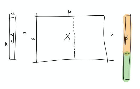
  • let’s just start with \(X\) and it’s covariance matrix \(\Sigma\): what we have here is something, at the population level, that can be described by a few large eigenvalues, and then many, many small eigenvalues. The idea is that the \(\Sigma\) describes the distribution of the sampled \(x\) vectors, and so the eigenvalues determine the variability in the direction of the respective engeinvector. However, there is no guarantee that there needs to be a rotation, so it is entirely possible that the variability in the \(x\)’s are concentrated on individual coordinates.
    • I incorrectly thought that what we have are random vectors, and so this spans all the coordinates, which makes it easier to extract the coefficients
  • So what we need are very many small directions of \(x\) (again, you can just align them to a coordinate)…
  • The optimal thing would be this nice sort of decomposition, where the first few elements of \(\beta\) correspond to the true coefficients. Then, the point is that the error can be entirely captured by a linear combination of the rest of the covariates.
  • 
  • This is a more explicit decomposition of the two terms
  • 
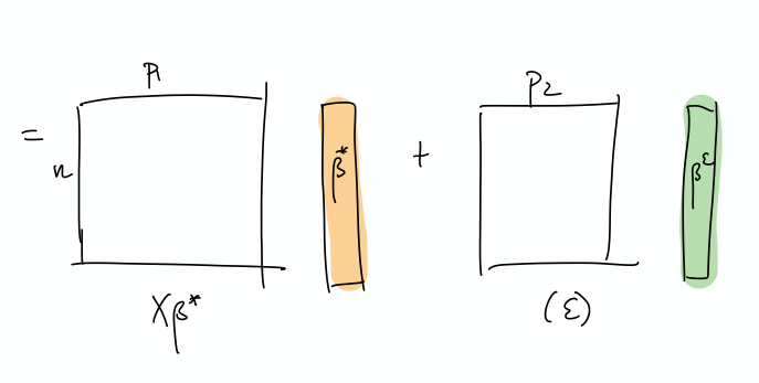
  • The idea here is that, in some simplified sense, the error is just a random Gaussian vector, and we should be able to represent it exactly as a linear combination of a lot of small gaussian vectors.

• classical statistics
  • bias/variance trade-off
  • model complexity
  • overfitting
• general principles:
  • you have a model, where you can tweak its model complexity: classic case of this is knn
    • I actually think that knn is problematic (though, I would have said the same thing about those nonparametric kernel regression methods)
    • essentially, the model “complexity” corresponds to basically being more “local”
    • in other words, complexity here can mean many things (maybe?)
    • perhaps the essence of the problem is the ability to have multiple solutions
      • though, again, that’s refuted by the kernel regression example, right?
  • intuition: you don’t want to go overboard with the model complexity, because at that point, you’ve overfit to the “training data”
  • ah right, there’s this other notion, of training/test and generalization:
    • this is a more difficult concept to pin down. basically, we think that the data comes from some “distribution” that’s going to be variable
    • if you could assume that the data you’re given is always correct, then perhaps you don’t mind too much about overfitting
    • though, even then, you still worry about overfitting in the sense that you don’t want to overfit on the training data (even aside from the noise problem)
  • let’s think of some simulations:
    • if you have noise, then you don’t really want to be overfitting
    • but even if you don’t have noise, you can still be worried about overfitting (is that true?)
      • that is, we usually like to assume some sort of smoothness to the function, which is really just an aesthetic (or an appeal to Occam’s Razor)
      • but perhaps the act of overfitting to the noise-less case will produce something a little too jagged
  • so we have training and test data, and the goal is to do better on the test data. even without looking at the test data, the intuition is that if you’ve gotten zero training error, then you’re probably doing something wrong.
    • one might think that if there is noise, then necessarily this must be true, since you’ve fit to the noise
    • but it seems like this depends on the flexibility of the model. that is, the model might be fitting to the noise, but it might be doing it in a very “weird” way, in that it localizes the effect of this training point
    • and if there is no noise, then you’re probably fine.
  • theory
    • as we talk about in class, you can basically perform this decomposition of the prediction error (at a point \(x\)) (wiki) in terms of
      • irreducible error (the noise in the data) \(\sigma^2\)
      • bias(\(f(x)\))
      • variance(\(f(x)\))
    • and so what i’m claiming is that, things are very different depending on the \(x\) that we’re considering
      • for \(x\) in the neighborhood of training points
        • we’re going to have low bias and high variance
      • but for \(x\) outside of those neighborhoods
        • we’re going to have the “optimal” trade-off (maybe?)
    • in this way, the decomposition doesn’t need to be thrown away - simply that the decomposition is now adaptive
      • this allows you to get zero training error, while still having optimal decomposition
    • alternative: paper (reviews) speculates that this is actually not a trade-off #paper
      • as you increase the width of neural networks, you get both reduction in variance and bias
      • I guess there isn’t any reason why these things must be opposed?
      • in principle, if your data is pretty straightforward, for instance,
        • something weird about all this is that, in my view, the irreducible error should somehow come into play here. as in, the generalizability of the model should be a function of the irreducible error?
  • classification vs regression (and the margin):

Let’s record the kinds of experimental data that we are interested in for [[project-interpolation]].

1. Replicating what’s been shown in the literature

• In the Zhang et al. (⊕2019Zhang, Chiyuan, Benjamin Recht, Samy Bengio, Moritz Hardt, and Oriol Vinyals. 2019. “Understanding deep learning requires rethinking generalization.” In 5th International Conference on Learning Representations, Iclr 2017 - Conference Track Proceedings. University of California, Berkeley, Berkeley, United States.) paper, they show that if you randomize the training data labels (in a classification problem), then you can still get zero training loss.
  • the point here is that the classical ideas of understanding the performance of machine learning methods (VC dimension) break down11 Though, I always get confused about this. Probably should reread one of the blog posts of Aroras..
• In some more recent work (Belkin et al. ⊕2019Belkin, Mikhail, Daniel Hsu, Siyuan Ma, and Soumik Mandal. 2019. “Reconciling modern machine-learning practice and the classical biasvariance trade-off.” Proceedings of the National Academy of Sciences 116 (32): 15849–54.), it was cited that if you randomize some of the training labels, you can basically still get the same generalization performance.
  • unclear to me if these two results are the same.
  • I vaguely remember there was some place that talked about the relevance to #robustness or #adversarial_training.
• establish that for standard problems (like CIFAR/MNIST/*), if you perturb the data (some percentage, or be clever about picking the points), then you’re going to maintain test performance.

2. New Ideas

• We conjecture that what’s going on is that there
  • show that this