#research
Testing a PA model
Testing Problem
We are interested in the following testing problem: how do we distinguish between a graph generated from a PA model, and a graph from a configuration model with the same degree distribution as the first graph?
The point of this test is, in part, to determine what are the defining properties of a PA model besides the fact that it is scale-free. Of course, we consider the undirected version, as otherwise it would be trivial (since PA vertices all have an out-degree of \(m\)).
Our first idea was to take inspiration from (Bubeck, Devroye, and Lugosi 2014Bubeck, Sébastien, Luc Devroye, and Gábor Lugosi. 2014. “Finding Adam in random growing trees.” arXiv.org, November. http://arxiv.org/abs/1411.3317v1.), and consider centroids1 defined as the vertex whose removal results in the minimum largest component. However, given the lack of an off-the-shelf implementation of this algorithm in R, we decided to look for a simpler test. As it turns out, if we just look at the nodes with the highest degree (together), we get interesting results.
set.seed(5)
library(igraph)
# create induced subgraph by taking the k largest degree nodes
create_induced_topk <- function(g, k) {
  n <- gorder(g)
  dg <- degree(g)
  induced_subgraph(g, order(dg)[(n-k+1):n])
}
# compares to graphs g,h to test which is which
tester <- function(g, h, k=20) {
  g2 <- create_induced_topk(g, k)
  h2 <- create_induced_topk(h, k)
  # if sizes are the same, we should return 1/2
  ifelse(gsize(g2) == gsize(h2), .5, gsize(g2) < gsize(h2))
}
Consider the following test: for a graph \(G\), calculate the induced subgraph by taking the top-\(k\) degree vertices. Which model produces an induced subgraph with more edges?
n <- 100
k <- 5
g <- sample_pa(n, power=1, m=2)
(g2 <- create_induced_topk(g, k))
## IGRAPH 99eb979 D--- 5 7 -- Barabasi graph
## + attr: name (g/c), power (g/n), m (g/n), zero.appeal (g/n), algorithm
## | (g/c)
## + edges from 99eb979:
## [1] 2->1 3->1 3->2 4->1 4->3 5->1 5->4h <- sample_degseq(degree(g), method="vl")
(h2 <- create_induced_topk(h, k))## IGRAPH bdfa659 U--- 5 6 -- Degree sequence random graph
## + attr: name (g/c), method (g/c)
## + edges from bdfa659:
## [1] 1--2 3--4 1--5 2--5 3--5 4--5par(mfrow=c(1,2))
Plot(g2)
Plot(h2)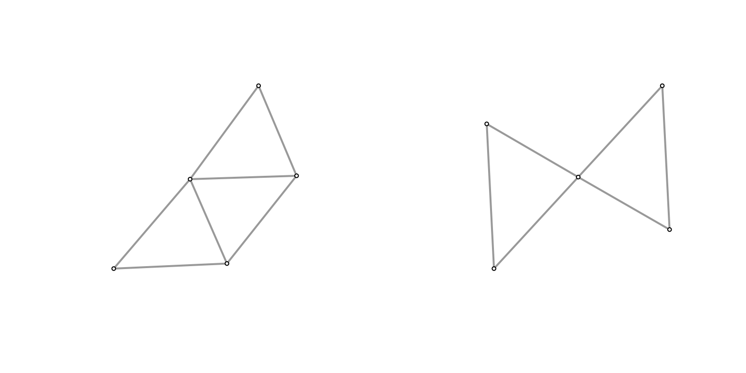
They don’t look that different at \((n,k) = (100,5)\), and the size of the graph is similar (edge count). What if we turn it up a notch?
n <- 1000
k <- 10
g <- sample_pa(n, power=1, m=2)
(g2 <- create_induced_topk(g, k))
## IGRAPH fdeb1f2 D--- 10 13 -- Barabasi graph
## + attr: name (g/c), power (g/n), m (g/n), zero.appeal (g/n), algorithm
## | (g/c)
## + edges from fdeb1f2:
## [1] 2->1 3->1 3->2 4->1 4->3 5->1 6->2 7->4 7->6 8->1 9->3 9->6
## [13] 10->3h <- sample_degseq(degree(g), method="vl")
(h2 <- create_induced_topk(h, k))## IGRAPH 1468645 U--- 10 22 -- Degree sequence random graph
## + attr: name (g/c), method (g/c)
## + edges from 1468645:
## [1] 1-- 3 2-- 3 1-- 4 2-- 4 3-- 4 1-- 5 2-- 5 1-- 6 2-- 6 4-- 6 3-- 7 4-- 7
## [13] 1-- 8 3-- 8 6-- 8 7-- 8 1-- 9 3-- 9 1--10 3--10 4--10 5--10par(mfrow=c(1,2))
Plot(g2)
Plot(h2)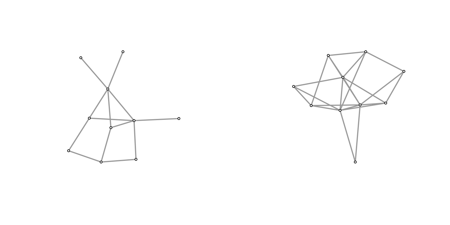
It feels like the induced subgraph from the configuration model is more densely connected (closer to a clique). Why might this be? In the case of the configuration model, if you consider the top \(k\) degree’d vertices, then there’s a very high probability of them being connected to one another2 if we take the half-edge formulation, then for any half-edge, it’s more likely to be connected to those with higher degrees (since they possess more half-edges). but they themselves have more half-edges, so it should amount to more edges between them.. Meanwhile, for a PA model, roughly we have that high degree nodes are older/earlier, and so probably have a slightly larger chance of connecting to each other than, say, a younger and an older node (since early on there aren’t many other options), but this is probably a much smaller effect.
To test this, let’s run some simulations. Here, I’ve run all combinations of \(n \in [100, 500, 1000]\) and \(k \in [5, 10, 15]\).
nsim <- 1000
ns <- c(100, 500, 1000)
ks <- c(5, 10, 20)
df <- expand.grid(k=ks, n=ns)
df$prob <- 0
cnt <- 1
for (k in ks) {
  for (n in ns) {
    res <- c()
    for (i in 1:nsim) {
      # generate graph
      g <- sample_pa(n, power=1, m=2)
      # generate the equivalent configuration model
      h <- sample_degseq(degree(g), method="vl")
      res <- c(res, tester(g, h, k=k))
    }
    df$prob[cnt] <- mean(res)
    cnt <- cnt + 1
  }
}
knitr::kable(df)| k | n | prob |
|---|---|---|
| 5 | 100 | 0.7475 |
| 10 | 100 | 0.8180 |
| 20 | 100 | 0.8705 |
| 5 | 500 | 0.9740 |
| 10 | 500 | 0.9940 |
| 20 | 500 | 0.9980 |
| 5 | 1000 | 0.9990 |
| 10 | 1000 | 1.0000 |
| 20 | 1000 | 1.0000 |
Clearly, we see a positive relationship between both \(k\) and \(n\) with respect to testing accuracy. Though, at \(n=1000\), it’s essentially as good as it’s going to get.
“Theory”
Here’s some hand-wavy calculations. For the simplest case of \(k=2\), we are interested in the probability that the top two degree vertices are connected. Let \(d_1, d_2\) be these degrees (and the respective vertex too). For the configuration model, for any given half-edge of \(d_1\), the probability that it’ll be connected to \(d_2\) is given by \(\dfrac{d_2}{D - d_1}\). Then, the probability that they’re connected is given, roughly, by \(\dfrac{d_1 \cdot d_2}{D}\).
Now consider the preferential attachment model. For now, let’s assume that \(d_1\) arrived before \(d_2\).3 can’t really WLOG here, but it feels close enough In other words, what we’re interested is the probability that one of the \(m\) vertices chosen by \(d_2\) was \(d_1\). Denote the arrival time4 which also corresponds to the number of vertices at that time of these two vertices as \(t_1\) and \(t_2\), respectively. Then, the probability is given by \(\dfrac{d_1(t_2)}{m \cdot t_2}\). The further out the \(t_2\), the larger the denominator, but also the more time \(d_1\) has had to amass its popularity.
The key is that it’s independent of \(d_2\) (i.e. the degree of the second vertex) – it would be the same probability for any other node at time \(t_2\).
Stewardship of Global Collective Beahvior
src: (Bak-Coleman et al. 2021Bak-Coleman, Joseph B, Mark Alfano, Wolfram Barfuss, Carl T Bergstrom, Miguel A Centeno, Iain D Couzin, Jonathan F Donges, et al. 2021. “Stewardship of global collective behavior.” Proc Natl Acad Sci USA 118 (27): e2025764118.)
A well written call-to-arms for some sort of interdisciplinary effort to understand the possible pernicious effects of social media and more broadly the rapid pace of technological change affecting the way we communicate, form groups, digest information, and hopefully provide guidance on how to solve these problems (e.g. writing pieces specifically for regulators).
They use a term called crisis discipline which I like, the canonical example being climate (change) science: you have this incredibly complicated system that needs urgent research and attention (for catastrophic reasons), but you don’t necessarily have the time (or it’s just not possible given the complexities of the system) to be entirely systematic and sure about the conclusions. In other words, these kinds of disciplines call for a much more agile form of research.
What’s interesting to me is that they couch all this talk through the lens of [[complexity-theory]]. The idea is that, for instance, once you connect half the world’s population together through the internet, or social media, you’re going to get unaccounted-for emergent behaviour, very much like those studied in complexity science, except usually the subject is natural processes (like swarms of locusts or school of fish). The difference now is that we’re dealing with humans, social interactions.
A good example here is the flow of information. Usually when we think of information flow we think of communication networks, where we’re sending bits of data around. However, the real information flow networks, and those that matter the most right now from a catastrophic perspective, are the information flows that we humans create when we read and share news over social media, thereby enabling the incredible propagation of fake news that we see permeate the world today. And this isn’t just a simple process: once you incorporate humans (and human judgement) into this network, it becomes infinitely more complicated to model and predict.
I definitely feel like this is something that I’ve been trying to articulate, and so I’m happy to see it laid out in this clear manner (unlike the way my brain organises its information, if it does that at all). It also has the same sort of flavor as my [[project-fairness]] work.
Dynamic Graph Models
The traditional way of thinking about networks is to treat them as essentially fixed, and samples from some generative model. Of course, we all know that networks don’t just spontaneously appear. That being said, a) collecting the entire history of a network’s evolution to its current state is often impossible, and b) dynamic models introduce too many more degrees of modelling freedom, so the purists generally shy away from it.
A useful dynamic model is one where the dynamics is fairly simple, and yet interesting global features still manifest themselves (in the spirit of [[complexity-theory]]). The classic example of this is the Preferential Attachment (PA) model, which, by a very simple rich-get-richer adjustment to the Uniform Attachment (UA) model creates a power-law degree distribution. A simple description of these models is, at each time step \(t\), we introduce a new vertex \(v_t\), and we add \(m\) new edges from this new one.1 i.e. each vertex has out-degree \(m\). The probability that an existing vertex has an edge to this vertex is either uniform (UA), or weighted by its current degree (PA),
\[ \begin{align*} P(A_{v_t, v_i}) = \frac{d_i}{\sum d_i}, \quad \forall i \in E. \end{align*} \]
Thanks to Bubeck, a completely different view of PA models is to focus on the temporal/growth aspect of it – by their very dynamics, we unlock a slew of different questions to ask. At a high level, the questions revolve around how much temporal information is recoverable from the final state?
For instance, we might be interested in determining the “seed” of a network2 You can adjust the model by starting with a fixed seed network (instead of a single node)., e.g. to figure out the early core of the internet. In the case of a pandemic, reverse-engineering the infection/contact network might give insight into the early actors. Of course, no real-life network follows a PA model exactly, which leads to the more practical question of, how much temporal information is recoverable even under a corrupted model?
A simple corruption is to simply inject random edges (sort of like having an ER graph embedded in the graph) – the opposite being having missing data (or both!). There’s probably an asymmetry here: adding edges makes retrieval more difficult than deleting edges. A simple extreme example: in the PA model with \(m=1\), the resulting graph is always a tree, which remains true when deleting but not when adding at random. Thus, any algorithm that relies on the tree breaks down.
Existing Work
The first problem (via this blog-post) involves asking questions about the seed graph (or the root). In a nutshell, the centroid of a tree, which is defined as the vertex whose removal results in the minimum largest component, is actually a good estimate of the root. Proving such a statement utilizes the probabilist’s favorite home appliance, the Polya Urn.
 Figure 1: The Centroid (1)
A similar problem (older blog-post) looks at the question of whether or not the seed graph has any influence (in the limit). Formally, we consider if the total variation distance between the two limiting distributions of two different seeds is bounded away from zero. This is a weaker requirement, since being able to recover the seed implies it has influence.
This line of inquiry can also be framed as follows: if we think about social networks, then what you might be interested in is this notion of the early-bird advantage – just by being there early, you get outsized returns (degree). Suppose people enter a network with the object of maximizing that return. Then it almost becomes something like a multilevel marketing (pyramid) scheme.
Open Problems
- Our intuition tells us that the network effect is definitely something that advantages people who are earlier to a platform. In a very similar vein to the rich-get-richer scheme, being early is essentially synonymous with being rich. However, it needn’t be that way. I think it might be useful to try to come up with a model that is essentially arrival-time agnostic, i.e. you have exchangeability at the node-level, which is something you generally get for free when you’re doing generative static network models, but is explicitly unavailable for dynamic models. Having such a model might help us elucidate the structural differences between two scale-free, dynamic models that differ on that one point.
Unsupervised Language Translation
Two papers:
- Word translation without parallel data. OpenReview (Conneau et al. 2017Conneau, Alexis, Guillaume Lample, Marc’Aurelio Ranzato, Ludovic Denoyer, and Hervé Jégou. 2017. “Word Translation Without Parallel Data.” arXiv.org, October. http://arxiv.org/abs/1710.04087v3.)
- Unsupervised Neural Machine Translation. OpenReview (Artetxe et al. 2017Artetxe, Mikel, Gorka Labaka, Eneko Agirre, and Kyunghyun Cho. 2017. “Unsupervised Neural Machine Translation.” arXiv.org, October. http://arxiv.org/abs/1710.11041v2.)
Unsupervised Neural Machine Translation
Typically for machine translation, it would be a supervised problem, whereby you have parallel corpora (e.g. UN transcripts). In many cases, however, you don’t have such data. Sometimes you might be able to sidestep this problem if there’s a bridge language where there does exist parallel datasets. What if you don’t have any such data, and simply monolingual data? This would be the unsupervised problem.
Figure 1: Architecture of the proposed system.

- They assume the existence of an unsupervised cross-lingual embedding. This is a key assumption, and their entire architecture sort of rests on this. Essentially, you form embedding vectors for two languages separately (which is unsupervised), and then align them algorithmically, so that they now reside in a shared, bilingual space.1 It’s only a small stretch to imagine performing this on multiple languages, so that you get some notion of a universal language space.
- From there, you can use a shared encoder, since the two inputs are from a shared space. Recall that the goal of the encoder is to reduce/sparsify the input (from which the decoder can reproduce it) – in the case of a shared encoder, by virtue of the cross-lingual embedding, you’re getting a language-agnostic encoder, which hopefully gets at meaning of the words.
- Again, somewhat naturally, this means you’re basically building both directions of the translation, or what they call the dual structure.
- Altogether, what you get is a pretty cute autoencoder architecture. Essentially, what you’re doing is training something like a [[siamese-network]]; you have the shared encoder, and then two separate decoders for each language. During training, you’re basically doing normal autoencoding, and then during inference, you just flip – cute!
- To ensure this isn’t a trivial task, they take the framework on the denoising autoencoder, and shuffle the words around in the input.2 I’m so used to bag-of-word style models, or even the more classical word embeddings that didn’t care about the ordering in the window, that this just feels like that – we’re harking back to the wild-wild-west, when we didn’t have context-aware embeddings. I guess it’s a little difficult to do something like squeeze all these tokens into a smaller dimension. However, this clearly doesn’t do that much – it’s just scrambling.
- The trick is then to adapt the so-called back-translation approach of (Sennrich, Haddow, and Birch 2016Sennrich, Rico, Barry Haddow, and Alexandra Birch. 2016. “Improving Neural Machine Translation Models with Monolingual Data.” In Proceedings of the 54th Annual Meeting of the Association for Computational Linguistics (Volume 1: Long Papers), 86–96. Berlin, Germany: Association for Computational Linguistics.) in a sort of alternating fashion. I think what it boils down to is just flipping the switch during training.
- Altogether, you have two types of mini-batch training schemes, and you alternate between the two. The first is same language (L1 + \(\epsilon\) -> L1), adding noise. The second is different language (L1 -> L2), using the current state of the NMT (neural machine translation) model as the data.
Word Translation Without Parallel Data
Figure 2: Toy Illustration

- With the similar constraint of just having two monolingual corpora, they tackle step zero of the first paper, namely how to align two embeddings (the unsupervised cross-linguagel embedding step). They employ adversarial training (like GANs).3 And in fact follow the same training mechanism as GANs.
- A little history of these cross-lingual embeddings: (Mikolov, Le, and Sutskever 2013Mikolov, Tomas, Quoc V Le, and Ilya Sutskever. 2013. “Exploiting Similarities among Languages for Machine Translation.” arXiv.org, September. http://arxiv.org/abs/1309.4168v1.) noticed structural similarities in emebddings across languages, and so used a parallel vocabulary (of 5000 words) to do alignment. Later versions used even smaller intersection sets (e.g. parallel vocabulary of aligned digits of (Artetxe, Labaka, and Agirre 2017Artetxe, Mikel, Gorka Labaka, and Eneko Agirre. 2017. “Learning bilingual word embeddings with (almost) no bilingual data.” In Proceedings of the 55th Annual Meeting of the Association for Computational Linguistics (Volume 1: Long Papers), 451–62. Vancouver, Canada: Association for Computational Linguistics.)). The optimization problem is to learn a linear mapping \(W\) such that4 It turns out that enforcing \(W\) to be orthogonal (i.e. a rotation) gives better results, which reduces to the Procrustes algorithm, much like what we used for the dynamic word embedding project. \[ W^\star = \arg\min_{W \in M_d (\mathbb{R})} \norm{ W X - Y }_{F} \]
- Given two sets of word embeddings \(\mathcal{X}, \mathcal{Y}\), the discriminator tries to distinguish between elements randomly sampled from \(W\mathcal{X}\) and \(\mathcal{Y}\), while the linear mapping \(W\) (generator) is learned to make that task difficult.
- Refinement step: the above procedure doesn’t do that well, because it doesn’t take into account word frequency.5 Why don’t they change the procedure to weigh points according to their frequency then? But now you have something like a supervised dictionary (set of common words): you pick the most frequent words and their mutual nearest neighbours, set this as your synthetic dictionary, and apply the Procrustes algorithm to align once again.
- It’s pretty important to ensure that the dictionary is correct, since you’re basically using that as the ground truth by which you align. Using \(k\)-NN is problematic for many reasons (in high dimensions), but one is that it’s asymmetric, and you get hubs (NN of many vectors). They therefore devise a new (similarity) measure, derived from \(k\)-NN: essentially for a word, you consider the \(k\)-NNs in the other domain, and then you take the average cosine similarity. You then penalize the cosine similarity of a pair of vectors by this sort-of neighbourhood concentration.6 Intuitively, you penalize vectors whose NN set is concentrated (i.e. it’s difficult to tell who is the actual nearest neighbor).
Post-Thoughts
It is interesting that these two papers are tackling the same, but different stages, of the NMT pipeline. In hindsight, it would have made much more sense to read the second paper first.
- Alternating minimization is a common strategy in many areas of computer science. For the most part (at least in academia), it’s application is limited by the difficulty
The Language of Animals
src: NewYorker, Earth Species.
This is a really interesting problem.
A Snide Comment about Certain Types of Research
While cleaning out my Dropbox account, I stumbled upon a collection of papers I had saved, almost a decade back. While browsing one of them (The Pulse of News in Social Media: Forecasting Popularity: arXiv), I couldn’t help notice parallels with the current papers I’m reading regarding [[project-misinformation]].
What’s funny is that back in 2012, the state of the art was well summarized by Figure 1. And this aligned almost exactly with what we were taught in our ML class. And now, of course, every paper is basically using neural networks, which again matches the state of the art.
 Figure 1: State of the Art in 2012!
I mean, at some level, this is just a comment about how ideas get circulated. Statistics and ML proffer methodologies that can then be applied to different problems to gain insight. It’s the natural sequence of events in science. At some other level, it sort of shows how derivative a lot of research really is. Of course, someone needs to apply the methods. And I guess people should be compensated for doing the labor (in the form of a publication).
I do think that something has changed in recent years. The flexibility of neural networks, and the need to play with the architecture, means that you can do cutting-edge research simply by trial and error. It has definitely moved more into the real of engineering. Another way to think about this is that, we used to worry about feature engineering, which is that you would spend a lot of time trying to create the right covariates to them input into your standard classification method. Now, we simply do feature-extraction engineering.