#src:paper

src: (⊕Hebart et al. 2020Hebart, Martin N, Charles Y Zheng, Francisco Pereira, and Chris I Baker. 2020. “Revealing the multidimensional mental representations of natural objects underlying human similarity judgements.” Nature Human Behaviour 4 (11): 1173–85.), and an earlier version in ICLR.

Contemplations

Distributed Representation

Figure 1: General Workflow

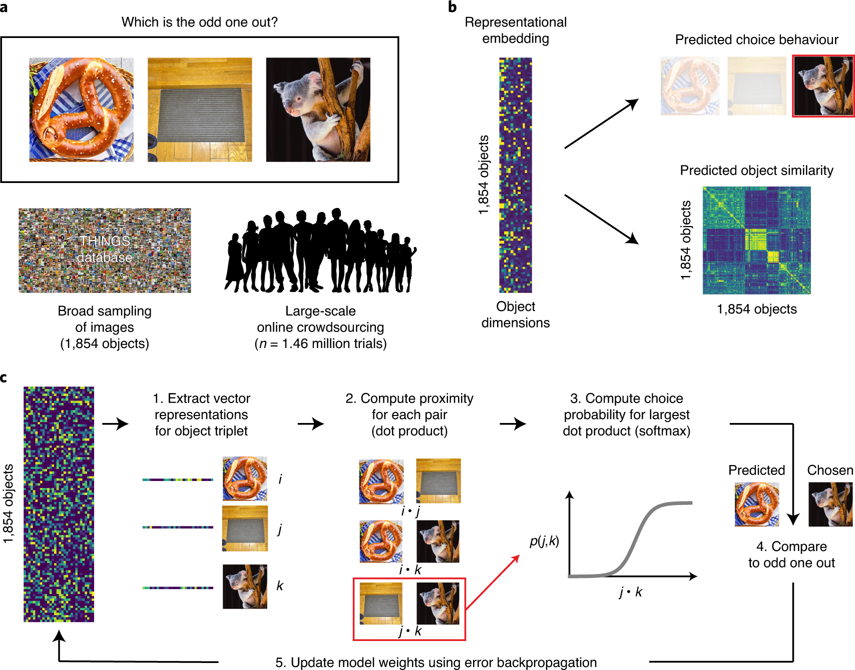
The idea of “distributed representation” (word2vec) is that a) words are represented as high-dimensional vectors, and b) words that cooccur should be closer together. What this means is that you can simply ingest a large corpus of unstructured text, collecting co-occurrence data, and learning a distributed representation along the way. The beautiful thing about this approach is that the only thing it relies on is some notion of co-occurrence; in the case of language, this is simply a window function.

What happens when you don’t have such information? Well then, you have to get a little creative. For those familiar with word2vec, you’ll know that a lesser-known but powerful trick they proposed is this notion of negative sampling: they found that it wasn’t enough to, during the traversal of your corpus and training your model, to push co-occurring words together, but it was also important to push words apart (i.e. randomly pick a word, and then do the opposite manoeuvre). Note the similarity to [[triplet-loss]]. In essense, we can move from pairs to triplets. But this seems like we’ve made the problem even more difficult.

As it turns out, the triplet structure allows us do something interesting, which is to turn the problem into an “odd-one-out” task. Cute!11 Dwelling on this a little longer, the paired version would be more like, show pairs to people and ask if they should be paired, which feels like an arbitrary task. The alternative, which is to give a rating of the similarity, naturally inherits all the ailments that come with analyzing ratings. In other words, given a corpus of images of objects, we can show a random triplet of them to humans, and ask which one is the odd one out. All that remains is to train our models with this triplet data. Here, they adapt softmax to this problem, applying it only to the chosen pair:

\[ \begin{align*} \sum_{(i,j,k)} \log \frac{ \exp\left\{ x_i^T x_j \right\} }{ \exp\left\{ x_i^T x_j \right\} + \exp\left\{ x_i^T x_k \right\} + \exp\left\{ x_j^T x_k \right\}} + \lambda \sum_{i = 1}^{m} \norm{x_{i}}_{1}, \end{align*} \]

where the first summation is over all triplets, but, crucially, we designate \((i,j)\) to be the chosen pair (i.e. \(k\) is the odd one out). The \(l_1\) penalty induces sparsity on the vectors, which improves intrepretability. Finally, and I’m not sure exactly how they implement this, but they also enforce the weights of the vector to be positive, to provide an additional modicum of interpretability.22 I feel like they overemphasize these two points, sparsity and positivity, as a way to differentiate themselves from other methods, when it’s really quite the trivial change from a technical perspective.

Figure 2: Interpretable dimensions

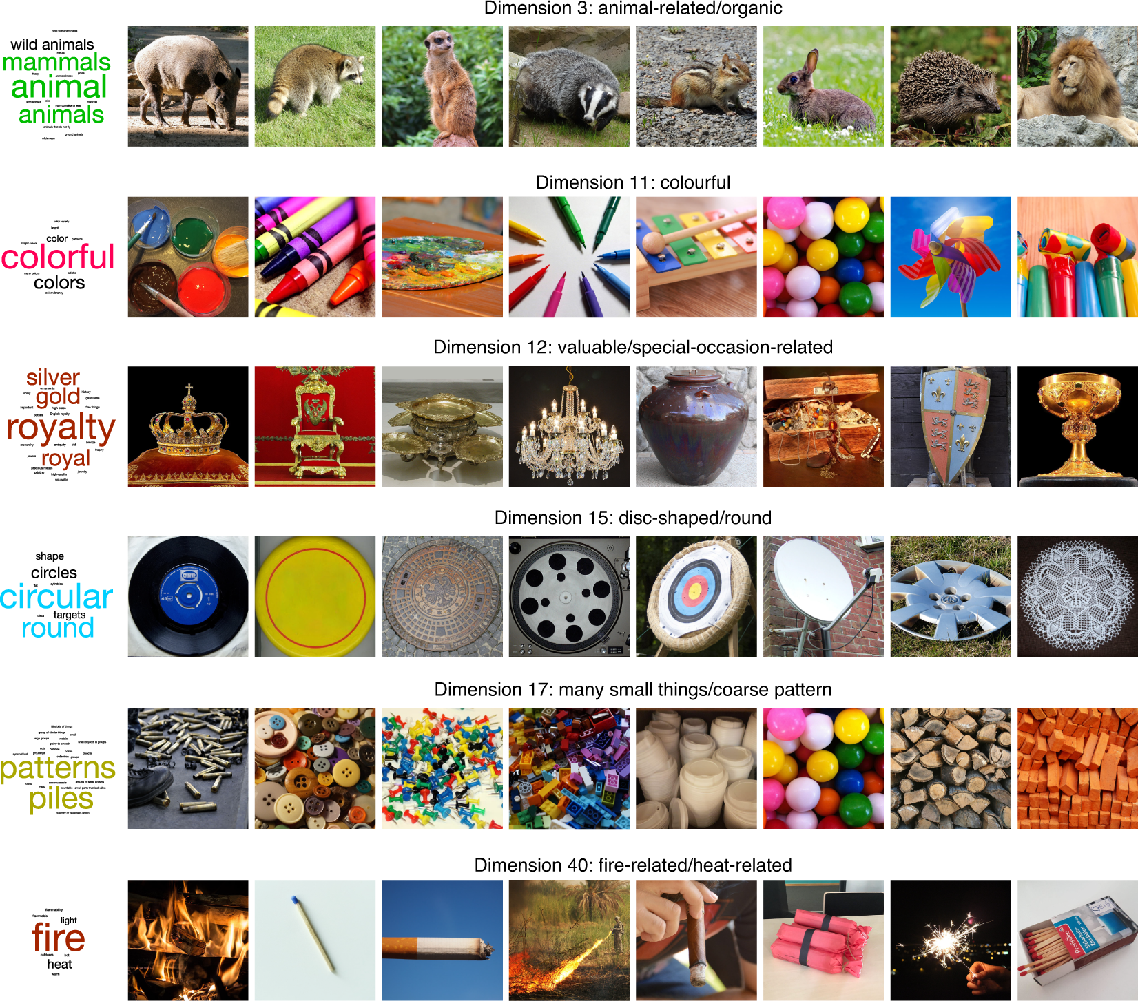
What is the output of this model? Ostensibly, it is a “distributed representation” of how we as humans organize our understanding of objects, albeit also conflating the particulars of the image used to represent this object.33 Does the prompt ask the subject to consider the image as an archetype, or simply ask to compare the three images on face value, whatever they see fit? My guess is probably the latter. Note that even though we’re dealing with the visual domain, the open-endedness of the task means that humans aren’t necessarily just using visual cues for comparison, but might also be utilizing higher order notions.

A crude approximation is that this model outputs two types of features: visual properties, like size, texture, etc.; and then the more holistic, higher-order properties, such as usage, value/price, etc. The key is that the latter property should not be able to be inferred from visuals alone.44 So really what I’m saying is that there are two groups, \(V\) and \(V^C\). Not groundbreaking. Thus, this model is picking something intangible that you cannot possibly learn from simply analyzing image classification models. However, this then begs the question: is it possible to learn a similar model by considering a combination of images (visual features) as well as text (holistic features)? What would be the nature of such a multi-modal learning model?

I see a few immediate challenges. The first is that, while one could take the particular image chosen in this experiment to represent an object, it would be too specific. What we would want is to be able to learn a single feature across all images of a single object. I feel like this should be something people have thought about, right? The second problem is, are word embedding of the objects sufficient to get the higher-order features? Supposing we solve all those problems, we’re still left with the question of how to combine these two things meaningfully. It feels to me like we should be training these things in unison?

Typicality

The idea here is that the magnitude of a particular dimension should import some meaning, the most likely being the typicality of this object to this particular feature (e.g. food-related). What they do is pick 17 broad categories (the graphs in Figure 3) that have a corresponding dimension in the vector representation, then for each image/object in this category (e.g. there are 19 images in the Drink category, corresponding to 19 points on the graph), they get humans to rate the typicality of that image for that category.

Figure 3: Typicality Scores

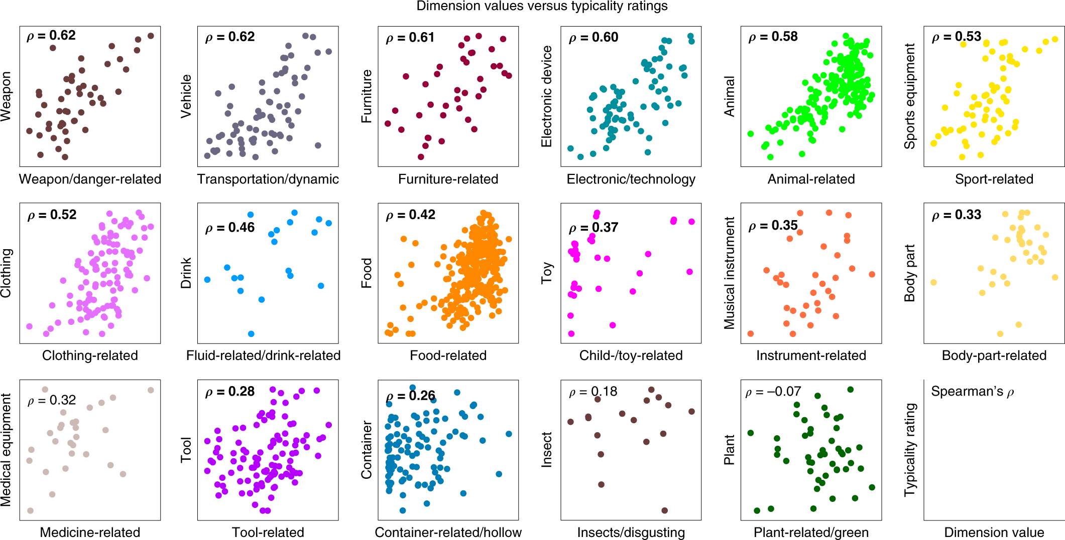
This result is somewhat surprising to me. For one, if you give me a list of images for, say, the category of animals, I would have no idea how to rate them based on typicality. Like, I think it would involve something cultural, regarding perhaps the stereotypes of what an animal is. I can imagine there being some very crude gradation whereby there are the clear examples of atypical, and then clear examples of typical, and then the rest is just a jumble. It doesn’t really appear that way from the data – I would have to look at these images to get a better sense.55 As an aside, I wish they also included the values of all the other images too, not just those in this category. Perhaps they are all at close to zero, which would be great, but they don’t mention it, so I assume the worst.

Also, how is it able to get at typicality through this model? I think what’s illuminating to note is that, out of the 27 broad categories of images in this dataset, 17 can be found in the 49-dimensional vector representation. Here’s what I think is probably happening (in particular for these 17 categories):

• if all three images are from different categories, then probably we’re learning something about one of those other dimensions (hopefully);66 Another thing is that this step helps to situate the categories amongst each other.
• if two images are from the same category, and the third is different, then the same pair is most often picked (helping to form this particular dimension);
• if all three images are picked, then I guess the odd one out is the one that’s the least typical.

Having laid it out like so, I’m starting to get a little skeptical about the results: it almost feels like this is a little too crude, and the data is not sufficiently expressive for a model to be able to learn something that’s not just trivial. Put another way, this almost feels like a glorified way of learning the categories – though, there’s nothing necessarily wrong with that, since the (high-level) categories are obviously important.

Perhaps it helps to consider the following generative model for images: suppose each image was represented by a sparse vector of weights, with many of the coordinates corresponding to broad categories. Set it up in a such a way that if you’re in a broad category, then that dominates all other considerations (so it follows the pattern above). Then, simply run this odd-one-out task directly on these vectors, and see if you’re able to recover these vectors.77 It almost feels like a weird autoencoder architecture…

src: (⊕Bak-Coleman et al. 2021Bak-Coleman, Joseph B, Mark Alfano, Wolfram Barfuss, Carl T Bergstrom, Miguel A Centeno, Iain D Couzin, Jonathan F Donges, et al. 2021. “Stewardship of global collective behavior.” Proc Natl Acad Sci USA 118 (27): e2025764118.)

A well written call-to-arms for some sort of interdisciplinary effort to understand the possible pernicious effects of social media and more broadly the rapid pace of technological change affecting the way we communicate, form groups, digest information, and hopefully provide guidance on how to solve these problems (e.g. writing pieces specifically for regulators).

They use a term called crisis discipline which I like, the canonical example being climate (change) science: you have this incredibly complicated system that needs urgent research and attention (for catastrophic reasons), but you don’t necessarily have the time (or it’s just not possible given the complexities of the system) to be entirely systematic and sure about the conclusions. In other words, these kinds of disciplines call for a much more agile form of research.

What’s interesting to me is that they couch all this talk through the lens of [[complexity-theory]]. The idea is that, for instance, once you connect half the world’s population together through the internet, or social media, you’re going to get unaccounted-for emergent behaviour, very much like those studied in complexity science, except usually the subject is natural processes (like swarms of locusts or school of fish). The difference now is that we’re dealing with humans, social interactions.

A good example here is the flow of information. Usually when we think of information flow we think of communication networks, where we’re sending bits of data around. However, the real information flow networks, and those that matter the most right now from a catastrophic perspective, are the information flows that we humans create when we read and share news over social media, thereby enabling the incredible propagation of fake news that we see permeate the world today. And this isn’t just a simple process: once you incorporate humans (and human judgement) into this network, it becomes infinitely more complicated to model and predict.

I definitely feel like this is something that I’ve been trying to articulate, and so I’m happy to see it laid out in this clear manner (unlike the way my brain organises its information, if it does that at all). It also has the same sort of flavor as my [[project-fairness]] work.

src: (⊕Bubeck and Sellke 2021Bubeck, Sébastien, and Mark Sellke. 2021. “A Universal Law of Robustness via Isoperimetry.” arXiv.org, May. http://arxiv.org/abs/2105.12806v1.)

Here’s another attempt to explain the overparameterization enigma found in deep learning (\(p >> n\)).

• to fit (interpolate) \(n\) data points of \(d\) dimensions, one requires \(nd\) parameters if one wants a smooth function (without the smoothness, \(n\) should suffice)
• thus, the overparameterization is necessary to ensure smoothness (which implies robustness)

Their theorem/proof works in the contrapositive: for any function class smoothly parameterized by \(p\) parameters (each of size at most \(\text{poly}(n,d)\)), and any \(d\)-dimensional data distribution satisfying mild regularity conditions, then any function in this class that fits the data below the noise level must have Lipschitz constant larger than \(\sqrt{\dfrac{nd}{p}}\).

• note that this result doesn’t say that you’ll fit a smooth function if you’re overparameterizing – just that if you don’t have enough parameters, then there’s no way you’re fitting a smooth one.
  • thus, in the context of scale (à la [[gpt3]]), this result says that scale is necessary to achieve robustness (though not sufficient).
• the noise level here is defined as the expected conditional variance \(\sigma^2 := \E[\mu]{\text{Var}(y \given x)} > 0\). noise is necessary from a theoretical perspective, as it prevents fitting a smooth classifier with perfect accuracy.

Two papers:

• Word translation without parallel data. OpenReview (⊕Conneau et al. 2017Conneau, Alexis, Guillaume Lample, Marc’Aurelio Ranzato, Ludovic Denoyer, and Hervé Jégou. 2017. “Word Translation Without Parallel Data.” arXiv.org, October. http://arxiv.org/abs/1710.04087v3.)
• Unsupervised Neural Machine Translation. OpenReview (⊕Artetxe et al. 2017Artetxe, Mikel, Gorka Labaka, Eneko Agirre, and Kyunghyun Cho. 2017. “Unsupervised Neural Machine Translation.” arXiv.org, October. http://arxiv.org/abs/1710.11041v2.)

Unsupervised Neural Machine Translation

Typically for machine translation, it would be a supervised problem, whereby you have parallel corpora (e.g. UN transcripts). In many cases, however, you don’t have such data. Sometimes you might be able to sidestep this problem if there’s a bridge language where there does exist parallel datasets. What if you don’t have any such data, and simply monolingual data? This would be the unsupervised problem.

Figure 1: Architecture of the proposed system.

1. They assume the existence of an unsupervised cross-lingual embedding. This is a key assumption, and their entire architecture sort of rests on this. Essentially, you form embedding vectors for two languages separately (which is unsupervised), and then align them algorithmically, so that they now reside in a shared, bilingual space.11 It’s only a small stretch to imagine performing this on multiple languages, so that you get some notion of a universal language space.
2. From there, you can use a shared encoder, since the two inputs are from a shared space. Recall that the goal of the encoder is to reduce/sparsify the input (from which the decoder can reproduce it) – in the case of a shared encoder, by virtue of the cross-lingual embedding, you’re getting a language-agnostic encoder, which hopefully gets at meaning of the words.
3. Again, somewhat naturally, this means you’re basically building both directions of the translation, or what they call the dual structure.
4. Altogether, what you get is a pretty cute autoencoder architecture. Essentially, what you’re doing is training something like a [[siamese-network]]; you have the shared encoder, and then two separate decoders for each language. During training, you’re basically doing normal autoencoding, and then during inference, you just flip – cute!
5. To ensure this isn’t a trivial task, they take the framework on the denoising autoencoder, and shuffle the words around in the input.22 I’m so used to bag-of-word style models, or even the more classical word embeddings that didn’t care about the ordering in the window, that this just feels like that – we’re harking back to the wild-wild-west, when we didn’t have context-aware embeddings. I guess it’s a little difficult to do something like squeeze all these tokens into a smaller dimension. However, this clearly doesn’t do that much – it’s just scrambling.
6. The trick is then to adapt the so-called back-translation approach of (⊕Sennrich, Haddow, and Birch 2016Sennrich, Rico, Barry Haddow, and Alexandra Birch. 2016. “Improving Neural Machine Translation Models with Monolingual Data.” In Proceedings of the 54th Annual Meeting of the Association for Computational Linguistics (Volume 1: Long Papers), 86–96. Berlin, Germany: Association for Computational Linguistics.) in a sort of alternating fashion. I think what it boils down to is just flipping the switch during training.
7. Altogether, you have two types of mini-batch training schemes, and you alternate between the two. The first is same language (L1 + \(\epsilon\) -> L1), adding noise. The second is different language (L1 -> L2), using the current state of the NMT (neural machine translation) model as the data.

Word Translation Without Parallel Data

Figure 2: Toy Illustration

1. With the similar constraint of just having two monolingual corpora, they tackle step zero of the first paper, namely how to align two embeddings (the unsupervised cross-linguagel embedding step). They employ adversarial training (like GANs).33 And in fact follow the same training mechanism as GANs.
2. A little history of these cross-lingual embeddings: (⊕Mikolov, Le, and Sutskever 2013Mikolov, Tomas, Quoc V Le, and Ilya Sutskever. 2013. “Exploiting Similarities among Languages for Machine Translation.” arXiv.org, September. http://arxiv.org/abs/1309.4168v1.) noticed structural similarities in emebddings across languages, and so used a parallel vocabulary (of 5000 words) to do alignment. Later versions used even smaller intersection sets (e.g. parallel vocabulary of aligned digits of (⊕Artetxe, Labaka, and Agirre 2017Artetxe, Mikel, Gorka Labaka, and Eneko Agirre. 2017. “Learning bilingual word embeddings with (almost) no bilingual data.” In Proceedings of the 55th Annual Meeting of the Association for Computational Linguistics (Volume 1: Long Papers), 451–62. Vancouver, Canada: Association for Computational Linguistics.)). The optimization problem is to learn a linear mapping \(W\) such that44 It turns out that enforcing \(W\) to be orthogonal (i.e. a rotation) gives better results, which reduces to the Procrustes algorithm, much like what we used for the dynamic word embedding project. \[ W^\star = \arg\min_{W \in M_d (\mathbb{R})} \norm{ W X - Y }_{F} \]
3. Given two sets of word embeddings \(\mathcal{X}, \mathcal{Y}\), the discriminator tries to distinguish between elements randomly sampled from \(W\mathcal{X}\) and \(\mathcal{Y}\), while the linear mapping \(W\) (generator) is learned to make that task difficult.
4. Refinement step: the above procedure doesn’t do that well, because it doesn’t take into account word frequency.55 Why don’t they change the procedure to weigh points according to their frequency then? But now you have something like a supervised dictionary (set of common words): you pick the most frequent words and their mutual nearest neighbours, set this as your synthetic dictionary, and apply the Procrustes algorithm to align once again.
5. It’s pretty important to ensure that the dictionary is correct, since you’re basically using that as the ground truth by which you align. Using \(k\)-NN is problematic for many reasons (in high dimensions), but one is that it’s asymmetric, and you get hubs (NN of many vectors). They therefore devise a new (similarity) measure, derived from \(k\)-NN: essentially for a word, you consider the \(k\)-NNs in the other domain, and then you take the average cosine similarity. You then penalize the cosine similarity of a pair of vectors by this sort-of neighbourhood concentration.66 Intuitively, you penalize vectors whose NN set is concentrated (i.e. it’s difficult to tell who is the actual nearest neighbor).

src: (⊕Roads and Love 2020Roads, Brett D, and Bradley C Love. 2020. “Learning as the unsupervised alignment of conceptual systems.” Nature Machine Intelligence 2 (1): 76–82.)

The surprising thing about * embeddings is that it relies solely on co-occurrence, which you can define however you want. This makes it a powerful generalized tool.11 And more generally, a key insight in statistical NLP is to not worry (too much) about the words themselves (except maybe during the preprocessing step, with things like stemming), but simply treat them as arbitrary tokens. For example, as in this paper, we can consider objects (or captions) of an image, and co-occurrence for objects that appear together in an image. From this dataset (Open Images V4: github), we can construct a set of embedding vectors (using GloVe) for the objects/captions (call this GloVe-img).

What is this set of embeddings? You can think of this as a crude learning mechanism of the world, using just visual data.22 Potential caveat (?): part of the data reflects what people want to take photos of, and be situated together. Though for the most part the objects in the images aren’t being orchestrated, it’s more just what you find naturally together. In other words, if a child were to learn through proximity-based associations alone, then perhaps this would be the extent of their understanding of the world.

A natural followup is, then, how does this embedding compare to the standard GloVe learned from a large text corpus?

At this point, I need to digress and talk about what this paper does:

• take the similarity matrix of the original GloVe vectors and the GloVe-img vectors. calculate the correlation of the matched entries. turns out that correlation can get as high as 0.3. perhaps that’s surprising?
  • seems like a waste to project things down to a similarity matrix. on the other hand, the arbitrariness of embeddings might make it difficult to compare embeddings directly.

src: NBER

One of the more fundamental changes of COVID-19, besides awareness of pandemics and the like, is a shift in the acceptance and future prevalence of WFH (and the consequences of a dramatic shift in people’s work habits).

We have seen a dramatic exodus of people in places like SF and NYC, which, pre-pandemic, was able to form a snowballing network effect, whereby having such a high concentration of talent and activity produced a self-perpetuating reality of ever-increasing rents and a matching demand for such rents. Entire ecosystems survived on catering to the maintenance and functioning of this concentrated enterprise, most of which effectively disappeared overnight.11 A while back there was a HN thread about whether or not the Silicon Valley folks that rely on this undercurrent of service (background) workers should support them during the pandemic. This sort of reminds me of the documentary we just watched, Sherpa, whereby it’s the Sherpas risking their lives, bringing the Westerner’s cargo and equipment to the next camp, that enables so many of them to ascend Mount Everest. Slightly different, since there we’re talking about people risking their lives, but given the almost subsistence-level income of these service workers, perhaps it isn’t too different. The key question is what is the permanent effect of this systemic shock (COVID-19) to such places?

The above paper, through longitudinal surveys, suggests that we’ll probably see more fractional WFH (i.e. generally better flexible working hours). On the other hand, it feels to me that this kind of flexibility is not actually the most efficient (unless you can reasonably predict rates). If everyone works from home, then you effectively do away with the office, perhaps transitioning to some kind of co-working/meeting space. If people are flexible, then your space requirements are at the whims of your employees, and so it becomes an optimization problem, with a penalty for going over-capacity. Obviously, providing the flexibility is a boon for individuals (more choice), but the best kinds of scenarios are win-win for everyone.

Frankly, I’m not qualified to talk much about the dynamics of office life (I doubt my life as an academic provides any insight there), as I have thus far managed to skirt such experiences. My experience with consulting provides personal evidence that, for certain kinds of jobs, with the right kind of people, a permanent WFH arrangement is entirely feasible. Though, again, things might change if everyone else in the team is working in the office. If you’re an employee, you’re definitely more likely to be passed up for promotions and the like.

Meanwhile, many people are dying to be back to the office. We’re lucky in that we have a large contingent at home, which keeps us sane and functioning. However, there’s the confounder of everyone simply being in lockdown – perhaps once everything opens up, people will prefer WFH when they can socialize during the other times.

src: (⊕Libby and Buschman 2021Libby, Alexandra, and Timothy J Buschman. 2021. “Rotational dynamics reduce interference between sensory and memory representations.” Nature Neuroscience.)

Cognition, our intelligence, lies, in part, in our ability to synthesize what we see before us (our sensory input) with our store of data (memory, maybe working, maybe long-term). In other words, intelligence is the cumulation of a time-cascade of information. Now, supposedly, due to the “distributed nature of neural coding,” this can lead to interference between the various time-levels.

This part is a little confusing to me, so let’s work through this slowly. Suppose we take a computer as an artificial example: you essentially have different stores of data with different read speeds (which loosely proxy sensory (registers), short-term (RAM) and long-term (disk)).11 In computers, the changing variable is read-speed/distance. Perhaps in the brain, the changing variable is the dimension of the data? Clearly, if you had enough “space,” there wouldn’t be an issue of interference. But of course our brains aren’t constructed to have simple, isolated stores,22 Well, we have neurons, and groups of neurons feel a little like discrete stores. This is where the limits of my knowledge are a crux; I feel like there are things like memory neurons, different templates of (perhaps groups of) neurons. On the other hand, the heavily architected memory components of the latest #deep_learning models cannot possibly be how the brain functions. We’re still missing the #biologically_inspired bit here. so perhaps it’s not even about the space constraint, but just the nature of the form of the “data.”

Figure 1: Computer Memory Pyramid

Let’s try and work backwards a little: why would our brains want to orthogonalize things? I think one of the key assumptions is that, for various reasons probably related to the protections afforded by redundancy and distributed representation (or even the noisy, arbitrary nature of life’s input), we represent information as high-dimensional vectors. Under this regime, then it really pays to utilize the whole space. How to do so? The most crude way would be to simply orthogonalize. But, actually, the fact that these vectors become orthogonal might just be a byproduct of some more complex process.

src: (⊕Chang and Tsao 2017Chang, Le, and Doris Y Tsao. 2017. “The Code for Facial Identity in the Primate Brain.” Cell 169 (6): 1013–1028.e14.), Nature news feature.

• primates have special(ized) face cells for disambiguation
• these cells are found in the inferotemporal (IT) cortex
  • two patches are considered: middle lateral/middle fundus (ML/MF), anterior medial (AM)
  • previous work showed a hierarchical relationship (AM being downstream, possibly the “final output stage of IT face processing”)
    • and \(\exists\) sparse set in AM which seemed to fire for specific individuals (independent of head orientation), suggesting it was capturing something very high-level
• question: what are the functions of these cells? one idea is that each cell encodes a particular individual11 “Jennifer Aniston” cells, after a study in epileptic patients found a cell that would only fire when presented with JA, regardless of face or just her name.
  • that does not scale, obviously22 I suspect that they just didn’t have a large enough sample. actually, that’s the whole point of this article! that just because it’s only firing for one thing in your set doesn’t necessarily mean it’s unique. one caveat might be that the things that would trigger activation might not be natural (so practically it’s unique). also, it’s important to distinguish visual/face processing, which is much more low-level, than, say, high-level object recognition, maybe.
• answer: construct the following face space:
  • decompose a face into two broad category of features
    • shape (S): i.e. the geometry of the facial landmarks
    • appearance (A): the rest (i.e. independent of shape)
      • this is accomplished by morphing all faces to the same average face-shape
  • from this decomposition, get 200 S and 200 A features, and perform PCA to get top 25 for each; giving, finally, a 50-d face space!
• result: single neurons are axis-coding (i.e. are projections in the face space)
  • to test this, simply determine the vector for a cell, and see faces that lie orthogonal to that vector have the same firing:
    • and crucially, they are able to determine the null space for those cells that were previously thought to be individual
  • 
  • similarly, they can predict response to new faces, which they also do.
• result: ML/MF cells fired more for shape, while AM fired more for appearance
• result: ~200 face cells needed to decode human faces (and encode)
• implications:
  • axis-coding, i.e. linear projections, are efficient, robust and flexible (see remark below).
• caveats:
  • all faces are neutral (i.e. don’t include expressions/emotions): but that seems fair, since we’re doing facial recognition, not emotion detection
  • potentially missing axes, given the training data

Thoughts:

• a point made in the paper is that this face space is rather constrained, and every point in this space is a valid/realistic face. however, that also suggests that it might be a little bit too restrictive
  • they’ve appreciated that other axes could be missing
  • but my worry is that, with results like “they can encode/decode faces,” the strong caveat there is: for faces falling into this particular space
    • granted, it is clearly a large space, but I suspect there are probably more axes available, and by projecting, you’re missing out on other spaces perhaps.
    • i.e. this is not necessarily the full picture
• a similar point is, it does feel like the features that they’ve come up with are closely related to the function of the cells, but I’m curious if a completely different encoding/feature-set would also produce the same empirical results
  • for instance, as they point out in the section of reproducing these results with a CNN, one doesn’t necessarily have to morph the face to get the appearance features (as it seems biologically implausible for our brains to be morphing faces)
  • and so they say you can probably get the same features by extracting information around the eyes
  • but then why not just do what we think the biology is doing
• a natural follow-up question is, what is the subspace spanned by these vectors: do they complete the space?
  • one would hope that the vectors themselves are orthogonal (or perhaps nearly orthogonal), though perhaps there’s redundancies inbuilt into the system (and perhaps the location of the cells might show that)

src: paper, via Michelle.

For the [[project-fairness]], we have been thinking in terms of algorithms and how to better design them to be better vanguards of such societal principles as equality. Something that I hadn’t thought about is the legal side of things; that is, what are the legal raminifications of introducing algorithms (and in the future, more powerful AI) to the legal process? If a judge’s decision rests on the results of an algorithm (e.g. criminal proceedings and giving bail), if lawyers themselves use algorithms for automating tasks (even creation of bills), or if it is the result of the algorithm in question that causes something persecutable (automated drones, self-driving cars) – these are all different examples of how AI might be part of the process.

The COMPAS debacle is a concrete example, and we saw the defendent argue that “the court’s use of the risk assessment violated his due process rights, in part because he was not able to assess COMPAS’s accuracy”. Clearly this is getting into legal territory – namely, what are his due process rights? What is sufficient for him to assess the accuracy?

The paper takes the view that explainable AI (xAI) is the answer to all this, and that it should be the judges (via the process of common law) that ought to decide the nature of the kinds of xAI that should be required depending on the circumstances. I don’t have much to say about the latter aspect of the thesis, as IANAL. However, my feeling is that this is just a much easier problem than the author makes it out to be; namely, just make it so that every algorithm is equipped with a full suite of xAI. It’s really not that difficult, and not much of an onus on the engineers. And one could go so far as require all closed-source algorithms have an open-source alternatives (or, as mentioned in the paper, I’m sure you can use existing legal structures involving confidential material).

This all feels like a red-herring to me though, and sidesteps the crux of the problem, which goes back to what I’ve been working on: the actual equitability or fairness of these algorithms. The idea is that, if you have xAI, and you can see the inner workings, then you can catch it doing bad things (which I agree), but if we’re going to be using algorithms, then we better actually be using justified algorithms before we apply them in court, at which point the xAI part of things is moot. For instance, if you were to show the defendent in the COMPAS example all the deconstructed analysis of the model, even right now there is no consensus among even academics about the fairness of the algorithm, how is this going to help anyone?

Also, the first thing that comes to my mind whenever we talk about xAI is that humans often have a hard time actually explaining their thought process – and yet, that has rarely stopped anyone in court. So part of this, I feel, is more a faith-in-humanity-more-than-machines type argument, which, as long as our prejudices are laid bare, I’m fine with that. Perhaps underlying that line of argument is the reasonableness or rationality of humans versus machines.11 This reminds me of how for self-driving cars, the bar is much higher when it comes to the level of safety before people feel comfortable. There’s this sort of weird disconnect between what we expect from AI, and what we expect from our fellow humans.

src: https://doi.org/10.1016/j.acap.2020.01.006

src: paper via EconTalk.

Using tools from extreme value theory (EVT), Cirillo and Taleb [1] determined that pandemics are patently fat tailed (with a tail exponent patently in the heaviest class: \(α < 1\)) — a fact that was well known (and communicated by Benoit Mandelbrot) but not formally investigated.

Pandemics are fat-tailed.

Random variables with unstable (and uninformative) sample moments may still have stable tail properties centrally useful for inference and risk taking.

RVs with undefined first (and second) moments are still parameterizable (e.g. Cauchy, and stable distributions).

From Wiki:

Many—notably Benoît Mandelbrot as well as Nassim Taleb—have noted this shortcoming of the normal distribution model and have proposed that fat-tailed distributions such as the stable distributions govern asset returns frequently found in finance.

For matters of survival, particularly when systemic, under such classes as multiplicative pandemics, we require “evidence of no harm” rather than “evidence of harm”.

Basically, if you have a fat-tailed distribution, and don’t have enough data to determine the properties of this particular sample, then expect the worst (since your sample moments are uninformative).

He then goes on to explain how, with fat-tailed distributions, confidence levels of the moments are too large to be practically useful (since second moments are so large).

src: (Tommasi et al. ⊕2015Tommasi, Tatiana, Novi Patricia, Barbara Caputo, and Tinne Tuytelaars. 2015. “A Deeper Look at Dataset Bias.” arXiv.org, May. http://arxiv.org/abs/1505.01257v1.)

Machine learning fundamentally operates by finding patterns in datasets.11 I always knew that datasets were biased (especially given the whole fairness problem), and this leads to various problems, but I didn’t realize this was a whole field of study. Fascinating. As such, the particulars of the dataset that you train on will affect what possible models can be learned.

Focusing on visual data for the moment, it is clear that, even while we are in the era of big data, most datasets cannot possibily capture every possible facet of visual information,22 which ties into the problem of self-driving cars whereby your dataset can’t possibly have every single possible circumstance, and thus it is these way off in the tail situations that cause the most headache, much like what people like Taleb always talk about. and so someone has to contend with the ways in which there are blind spots or biases as a result of the particular curation of data.

Causes:

• capture bias: thigs like POV, lighting condition, actual device used;
• label bias: this is mainly a problem with supervised learning, as you often have explicit labels (maybe with a bounding box), and there is no notion of ambiguity or subtlety in the labels;
• negative bias: which again is about supervised learning and simply noting all other possible categories not in the dataset.

So now we know that we have all these problems with the coverage of the dataset. Ultimately though, the actual thing we care about is generalization performance, or basically how well this does out-of-sample. After all, even if your model has all these issues, if it is intelligent enough to do well on out-of-sample things, then its sort of a moot point.

Key terms:

• domain shift: general term to describe the fact that the training data probability model \((X,Y)\) changes from train to test. In particular, it encompasses changes in \(P(Y \given X)\), \(P(X)\) or even \(P(Y,X)\).
• covariate shift: when the distribution of the covariates change
  • theory: source (\(S\)) and target (\(T\)) operate in the same space (\(X\) input, \(Y\) output). conditional distributions are the same: \(P_S(Y \given X) = P_T(Y \given X)\) (which essentially says that the model is intact); but marginal distribution has changed: \(P_S(X) = P_T(X)\).
• sample selection bias: same thing as covariate shift?? in my mind sample selection bias is more specific case of covariate shift, that happens as a result of improper selection, whereas covariate shift can be something natural.
• class imbalance: specific to classification, when you have poorly represented classes (so here we’re talking about the \(Y\)’s)

src: (Breiman ⊕2001Breiman, L. 2001. “Statistical modeling: The two cultures.”)

Written in 2001, I would say that many of the issues raised in this seminal paper have not changed much in the intervening years.

via blog and (Li and Arora ⊕2019Li, Zhiyuan, and Sanjeev Arora. 2019. “An Exponential Learning Rate Schedule for Deep Learning.” arXiv.org, October. http://arxiv.org/abs/1910.07454v3.)

Two key properties of SOTA nets: normalization of parameters within layers (Batch Norm); and weight decay (i.e \(l_2\) regularizer). For some reason I never thought of BN as falling in the category of normalizations, ala [[effectiveness-of-normalized-quantities]].

It has been noted that BN + WD can be viewed as increasing the learning rate (LR). What they show is the following:

The proof holds for any loss function satisfying scale invariance: \[ \begin{align*} L(c \cdot \theta) = L(\theta) \end{align*} \] Here’s an important Lemma:

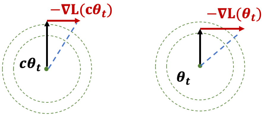Figure 1: Illustration of Lemma

The first result, if you think of it geometrically (Fig. 1), ensures that \(|\theta|\) is increasing. The second result shows that while the loss is scale-invariant, the gradients have a sort of corrective factor such that larger parameters have smaller gradients.

src: blog version of paper.

Learning a DAG is essentially a #causal_inference problem, with the key being that the graph has to be acyclic. But this type of problem is generally NP-hard. These people came up with a continuous version of the constraint, taking advantage of matrix exponentials.

src: (Feldman ⊕2019Feldman, Vitaly. 2019. “Does Learning Require Memorization? A Short Tale about a Long Tail.” arXiv.org, June. http://arxiv.org/abs/1906.05271v3.)

A different take on the interpolation/memorization conundrum.

The key empirical fact that this paper rests on is this notion of data’s long-tail.11 This was all the rage back in the day, with books written about it. Though that was more about #economics and how the internet was making it possible for things in the long tail to survive. Formally, we can break a class down into subpopulations (say species22 Though they don’t have to be some explicit human-defined category.), corresponding to a mixture distribution with decaying coefficients. The point is that this distribution follows a #power_law distribution.

Now consider a sample from this distribution (which will be our training data). You essentially have three regimes:

1. Popular: there’s a lot of data here, you don’t need to memorize, as you can take advantage of the law of large numbers.
2. Extreme Outliers: this is where the actual population itself is already incredibly rare, so it doesn’t really matter if you get these right, since these are so uncommon.
3. Middle ground: this is middle ground, where you still might only get one sample from this subpopulation, but it’s just common enough (and there are enough of them) that you want to be right. And since they’re uncommon, you basically only have one copy anyway, so your best choice is to memorize.

Key: a priori you don’t know if your samples are from the outlier, or from the middle ground. So you might as well just memorize.33 What you have is that actually, what you don’t mind is selective memorization. Though it’s probably too much work to have two regimes, so just memorize everything.

My general feeling is that there is probably something here, but it feels a little too on the nose. It basically reduces the power of deep learning to learning subclasses well, when I think it’s more about the amalgum of the whole thing.

src: link

• Actually does Local Testing on Graphs, as I’ve wanted to do. But in a very simple manner. Basically, you define dyadic imbalance as the fraction of cycles that are unbalanced. Cool.
• they also basically handle multiplex networks by essentially merging everything into one graph. Cool.
• data
  • what is sort of interesting is their application to IR is quite extensive (and very different to the social network setting)
  • they also have something related to voting decisions in the US Congress, which seems pretty interesting (like Wikipedia admin voting)
• method
  • they use the permutation test (which they explain in a very roundabout way)
  • they use something called a Heckman Selection Model, which I highly doubt solves the problem, but maybe it does?
    • this is some model that claims to fix sample selection biases
  • basically, they treat it like a covariate. but this is where we might be able to show something bad about their model. Basically, just like the whole spurious test when running linear regression on time series, doing node covariate regression, especially when you have graph statistics that are highly dependent is going to screw you over

src: arXiv

• defines the Generalization Gap: DNNs generalize better when trained with smaller batch sizes
  • i.e. SGD good
• characterize the various regimes of the eigenvalue distribution
  • very much similar to the Wigner’s Semi-Circle Law, distribution of eigenvalues from a random matrix
  • if the elements of the random matrix are correlated, you don’t get the same behavior, but something more heavy-tailed
• capacity-control
  • use some form of “rank” to describe the capacity of the learned DNN
• findings:
  • as you decrease batch-size, you get different behavior of the singular values, more “regularized”, corresponding to more “correlated” random-matrices
  • what they roughly show is that, during training, you’re effectively reducing the rank
    • more precisely, they go through the 5 stages of distribution of eigenvalues
    • and this clearly translates into something about the rank (since in the heavy tail, then things can escape the main body)
• implications:
  • by having smaller sizes, it’s able to detect more correlations (?), and as a result, you get the whole heavy-tailed distribution
    • importantly, that leads to better rank (?). this must have something to do with rank.
  • The obvious mechanism is that, by training with smaller batches, the DNN training process is able to “squeeze out” more and more finer-scale correlations from the data, leading to more strongly-correlated models. Large batches, involving averages over many more data points, simply fail to see this very fine-scale structure, and thus they are less able to construct strongly-correlated models characteristic of the Heavy-Tailed phase.

src: (Bartlett et al. ⊕2020Bartlett, Peter L, Philip M Long, Gábor Lugosi, and Alexander Tsigler. 2020. “Benign overfitting in linear regression.” Proceedings of the National Academy of Sciences of the United States of America vol. 80 (April): 201907378.).

• references:
  • slides, better exposition
  • new paper that generalizes this: “Benign overfitting in the large deviation regime”, via arXiv
• setting:
  • linear regression (quadratic loss), linear prediction rule
    • important: we are actually thinking about the ML regime, whereby there isn’t just a true parameter, but that there is a best one by considering the expectation (which, under general settings, corresponds to what would be the “truth”).
    • important: they are considering random covariates in their analysis! I guess this is pretty standard practice, when you’re calculating things like risk
    • that is, you can think of linear regression as a linear approximation to \(\mathbb{E} ( Y_i \,\mid\, X_i)\)
    • blog with a good explanation: very standard classical exposition, showing that the conditional expectation is the optimal choice for \(L_2\) loss, and the linear regression solutions is the best linear approximation to the conditional expectation (something like that)
  • infinite dimensional data: \(p = \infty\) (separable Hilbert space)
    • though results apply to finite-dimensional
  • thus, there exists \(\theta^*\) that minimizes the expected quadratic loss
    • in order to be able to calculate expected value, they must be assuming some model (normal error)
  • but they want to deal with the interpolating regime, so at the very least \(p > n\), and probably >>
  • “We ask when it is possible to fit the data exactly and still compete with the prediction accuracy of \(\theta^*\).”
    • Unless I’m being stupid, this line doesn’t make any sense. If you fit the data exactly, then by definition you’re an optimal solution
  • the solution that minimizes is underdetermined, so there isn’t a unique solution to the convex program
  • okay, so I think what they’re trying to say is that, if your choice of \(\hat{\theta}\) is the one that minimizes the quadratic loss (= 0), and then pick the one with minimum norm (what norm), then let’s see when do you get good generalizability
  • “We ask when it is possible to overfit in this way – and embed all of the noise of the labels into the parameter estimate \(\hat{\theta}\) – without harming prediction accuracy”
• results:
  • covariance matrix \(\Sigma\) plays a crucial role
  • prediction error has following decomposition (two terms):
    • provided nuclear norm of \(\Sigma\) is small compared to \(n\), then \(\hat{\theta}\) can find \(\theta^*\)
    • impact of noise in the labels on prediction accuracy (important)
      • “this is small iff the effective rank of \(\Sigma\) in the subspace corresponding to the low variance directions is large compared to \(n\)”
  • “fitting the training data exactly but with near-optimal prediction accuracy occurs if and only if there are many low variance (and hence unimportant) directions in parameter space where the label noise can be hidden”
• intuition: I don’t think they’ve provided much in the way of any intuition about what is going on, so let’s see if we can come up with some
  • this is weird because we’re thinking of linear regression, and so basically it’s a linear combination of the \(X\)’s to get \(Y\).
  • if we were to think about this geometrically, is that we have an infinite dimensional \(C(X)\), with sufficient “range”/span that our \(Y\) lands in \(C(X)\).
  • I feel like what they’re trying to do is basically have the main true linear model, and then what you have are these small vectors in all sorts of directions, so that you can just add those to your solution, in order to interpolate (??)
    • and since we’re dealing with a model that is linear in truth, then
    • I’m confused, because since both \(x,y\) are random, then calculating the risk is over both of these things.
• takeaway:
  • basically, the eigenvalues of the covariance matrix should satisfy:
    • many non-zero entries, large compared to \(n\)
    • small sum compared to \(n\) (smallest eigenvalues decays slowly)
    • i.e. lots of small ones, probably some big ones (?)
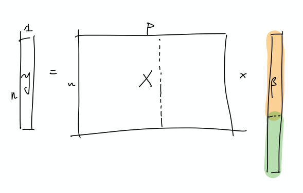
• summary: this is what I think is going on
  • let’s just start with \(X\) and it’s covariance matrix \(\Sigma\): what we have here is something, at the population level, that can be described by a few large eigenvalues, and then many, many small eigenvalues. The idea is that the \(\Sigma\) describes the distribution of the sampled \(x\) vectors, and so the eigenvalues determine the variability in the direction of the respective engeinvector. However, there is no guarantee that there needs to be a rotation, so it is entirely possible that the variability in the \(x\)’s are concentrated on individual coordinates.
    • I incorrectly thought that what we have are random vectors, and so this spans all the coordinates, which makes it easier to extract the coefficients
  • So what we need are very many small directions of \(x\) (again, you can just align them to a coordinate)…
  • The optimal thing would be this nice sort of decomposition, where the first few elements of \(\beta\) correspond to the true coefficients. Then, the point is that the error can be entirely captured by a linear combination of the rest of the covariates.
  • 
  • This is a more explicit decomposition of the two terms
  • 
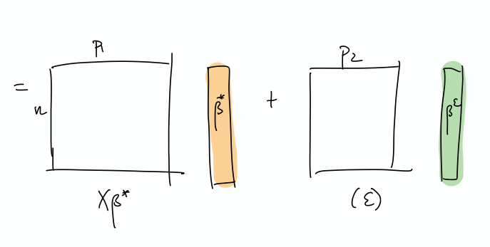
  • The idea here is that, in some simplified sense, the error is just a random Gaussian vector, and we should be able to represent it exactly as a linear combination of a lot of small gaussian vectors.

(⊕Blalock et al. 2020Blalock, Davis, Jose Javier Gonzalez Ortiz, Jonathan Frankle, and John Guttag. 2020. “What is the State of Neural Network Pruning?” arXiv.org, March. http://arxiv.org/abs/2003.03033v1.): NN pruning is an iterative method whereby you train a network (or start with a pre-trained model), prune based on assigned scores to structures/parameters, then retrained (since the pruning step will usually reduce accuracy), which is known as fine-tuning.

src: (Arora, Cohen, and Hazan ⊕2018Arora, Sanjeev, Nadav Cohen, and Elad Hazan. 2018. “On the optimization of deep networks: Implicit acceleration by overparameterization.” In 35th International Conference on Machine Learning, Icml 2018, 372–89. Institute for Advanced Studies, Princeton, United States.), section 3 on \(l_p\) regression

They show that in the simple scalar linear regression problem, i.e. loss function

\[ \begin{align*} \E[(x,y)\sim S]{\frac{1}{p}(y - \mathbf{x}^\top \mathbf{w})^p} \end{align*} \]

if you overparameterize ever so slightly to

\[ \begin{align*} \E[(x,y)\sim S]{\frac{1}{p}(y - \mathbf{x}^\top \mathbf{w}_1 w_2)^p}, \end{align*} \]

then gradient descent turns into an accelerated version.

• I remember Arora presenting on this particular result a few years back (or something like this), and finding it very intriguing.
• I think this goes nicely with the theme of [[statistics-vs-ml]], though it’s a slightly different angle.
  • essentially: we statisticians are afraid of overparameterization, because it removes specificity/leads to ambiguity
  • but actually, when it comes to these gradient methods, it actually helps to overparameterize

src: (Arora, Cohen, and Hazan ⊕2018Arora, Sanjeev, Nadav Cohen, and Elad Hazan. 2018. “On the optimization of deep networks: Implicit acceleration by overparameterization.” In 35th International Conference on Machine Learning, Icml 2018, 372–89. Institute for Advanced Studies, Princeton, United States.)

• question: what role does depth play in deep learning?
• idea: depth is an accelerator
  • somehow incorporates momentum
• how to check, though. depth plays two roles:
  • better representation power
  • overparameterization (changing the landscape, ish)
    • and not just via width, but via depth
• solution: consider linear neural networks, so that expressiveness is fixed11 This is a cute justification for linear neural networks.
• results:
  • show depth is equivalent to shallow (1-layer) + preconditioner
    • that essentially combines momentum
  • and that this acceleration cannot be replicated via gradient descent + regularizer
    • though does not discount the possibility of an accelerated version
    • this proof felt a little spurious [[troubling-trends-in-machine-learning-scholarship]]
• subtleties:
  • this is for generic loss function (convex?), no longer just about matrix completion (I worked backwards)

offshoot: [[overparameterized-regression]]

src: (Lipton and Steinhardt ⊕2019Lipton, Zachary, and Jacob Steinhardt. 2019. “Troubling Trends in Machine Learning Scholarship.” Queue, February.)

src: arXiv

src: slides

Setup

In a linear network, we have \(N\) matrices (weight matrices, parameters), the product of which \(W_N \ldots W_1 = W_{1:N}\) we call the end-to-end matrix. This is what we use in the loss function.

Note that when we actually calculate the gradient, we’re going to be doing it for all the individual matrices/parameters. But it turns out that there’s an equivalence between this natural gradient flow (what actually gets implemented), and the one if you were to consider the single-layer version.

Figure 1: Comparison between the two equivalent linear models

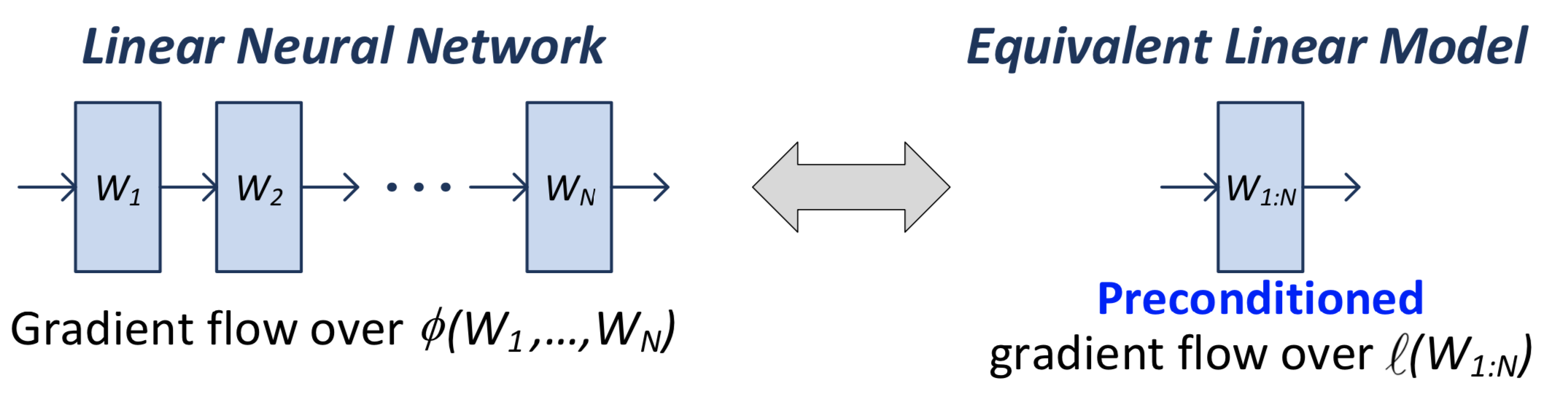
What you can show is that the gradient flow of the \(W_{1:N}\) matrix is equivalent to a pre-conditioned version of the single-layer gradient:

\[ \begin{equation} \frac{d}{dt} \operatorname{vec}\left[ W_{1:N}(t) \right] = - P_{W_{1:N}(t)} \cdot \operatorname{vec}\left[ \nabla l( W_{1:N}(t)) \right] \tag{1} \end{equation} \]

Thus, adding additional (redundant) linear layers induces “preconditioners promoting movement in directions already taken”.[^ Preconditioners are linear transformations that condition a problem to make it more suitable for numerical solutions, and usually involve reducing the condition number. It turns out that the ideal preconditioner is the M-P pseudo-inverse, which we’ve seen before, [[pseudo-inverses-and-sgd]].]

Recall that the condition number is the ratio of the max to the min singular value, so relates to how much the matrix scales the input.

Important: this above analysis (1) is independent of the form of the loss function. I think the only requirement is that the parameters come into the loss function through the end-to-end matrix.