202005152209
Matrix Completion Experiments
tags: [ proj:penalty , experiments ]
For posterity, we leave some of our experiments up.
Comparison of various matrix completion methods, in the noise-less case. I did 5 repeats, so the first graph is with all repeats, while the second graph is mean-collapsed. The Convex Program actually does really well (it’s just slow, probably at the same order as our LNN).
library(ggplot2)
x <- read.csv("20-05-17 comparison.csv")
ggplot(x, aes(x=sample_size, y=Loss.test, group=method)) + geom_point() + geom_smooth() + scale_y_log10() + facet_grid(.~method)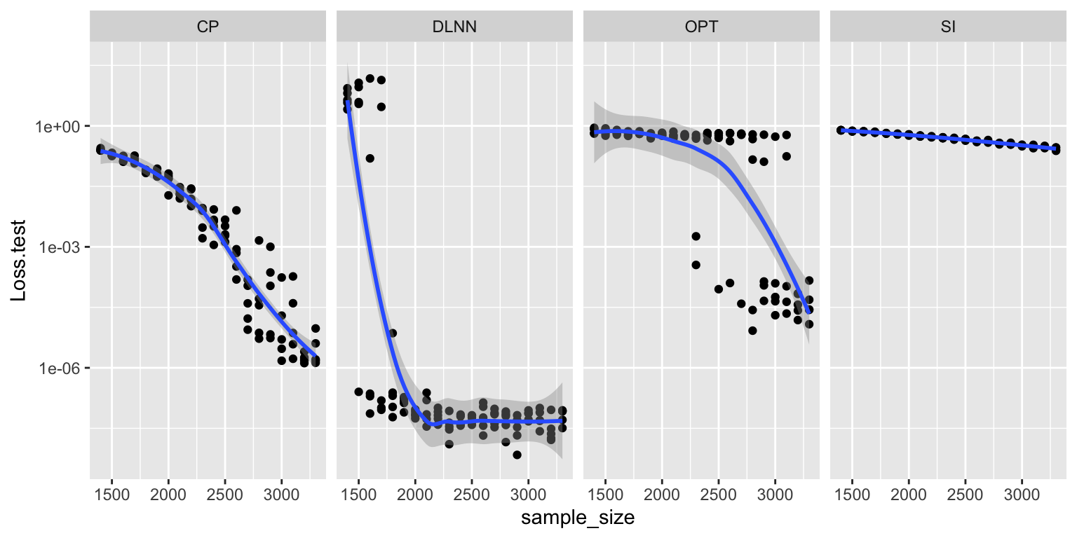
y <- aggregate(x$Loss.test, list(sample_size=x$sample_size, method=x$method), mean)
ggplot(y, aes(x=sample_size, y=x, color=method)) +
  geom_point() +
  geom_line() +
  scale_y_log10() +
  # geom_smooth(method = lm, formula = y ~ splines::bs(x, 3), se = FALSE) +
  ylab("test loss")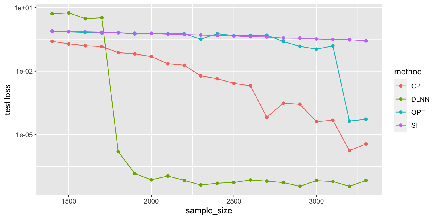
Adding Noise
The curious thing is that, things become much more equal when you introduce noise.
x <- read.csv("comparison2.csv")
x[x$method=="DLNN", "method"] = "Adam:2 (ratio)"
z <- read.csv("20-05-18 comparison.csv")
z$method <- ifelse(z$optim=="Adam", "Adam:4 (ratio)", "GD:4 (ratio)")
z2 <- read.csv("20-05-19 comparison.csv")
z2$method <- ifelse(z2$reg_norm=="ratio", "GD:4 (n/a)", "GD:4 (nuc)")
z <- z[,names(x)]
z2 <- z2[,names(x)]
x <- rbind(x,z,z2)
y <- aggregate(x$Loss.test, list(sample_size=x$sample_size, method=x$method, noise=x$noise), mean)
ggplot(y, aes(x=sample_size, y=x, color=method)) + geom_line() + scale_y_log10() + facet_grid(.~noise) + ylab("test loss")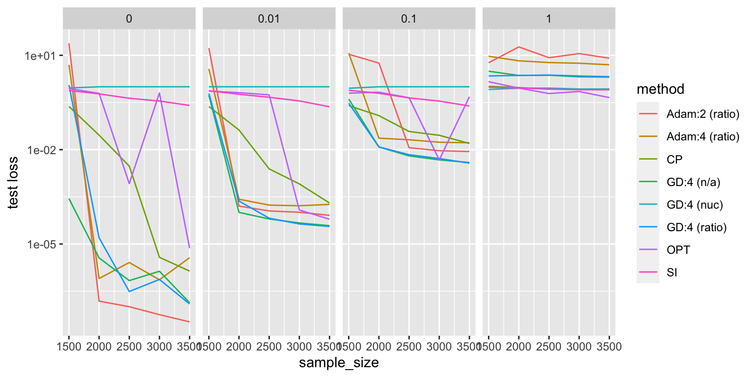
- gradient descent with or without the penalty does really well, especially with a little bit of noise
- interestingly, things reverse with enough noise. in the panel where \(\sigma = 1\), all the neural network methods are dominated by the other methods
- at zero noise, things are the opposite
- with nuclear penalty, everything is just terrible
- curious: it looks like there’s almost a phase transition in sample size for Adam. maybe it just needs more sample size to get to the same rate.
Remarks:
- it feels like noise is somehow equalizing the playing field. put another way, it’s sort of masking the problem at hand.
- there’s the recovery of the low-rank matrix from the observations, and then there’s figuring out, accounting for noise, which low-rank matrix in the vicinity should you choose.
- this relates (nicely) to [[project-interpolation]]. here, we are dealing with depth of 2, and so one could argue that we’re in the regime where we’re just able to interpolate, but not well enough, so you can’t get nice generalization.
- but it feels like matrix completion is a very particular problem, and since we’re restricting ourselves to just linear neural networks, I don’t expect to see the same kind of double-dipping behaviour.
- if we relax the loss function (have it within \(\delta\)), we should be able to get competitive rates in the noisy case? [[idea]]
Update
For some reason, we never tried depth 1!
z3 <- read.csv("20-05-20 comparison.csv")
z3$method <- ifelse(z3$optim=="Adam", "Adam:1 (ratio)", "GD:1 (ratio)")
z3 <- z3[,names(x)]
x <- rbind(x,z3)
y <- aggregate(x$Loss.test, list(sample_size=x$sample_size, method=x$method, noise=x$noise), mean)
y <- y[stringr::str_detect(y$method, "\\("),]
y <- y[!stringr::str_detect(y$method, "(nuc|n/a)"),]
y$GD <- stringr::str_detect(y$method, "GD")
ggplot(y, aes(x=sample_size, y=x, color=method)) + geom_line(aes(linetype=GD)) + scale_y_log10() + facet_grid(.~noise) + ylab("test loss")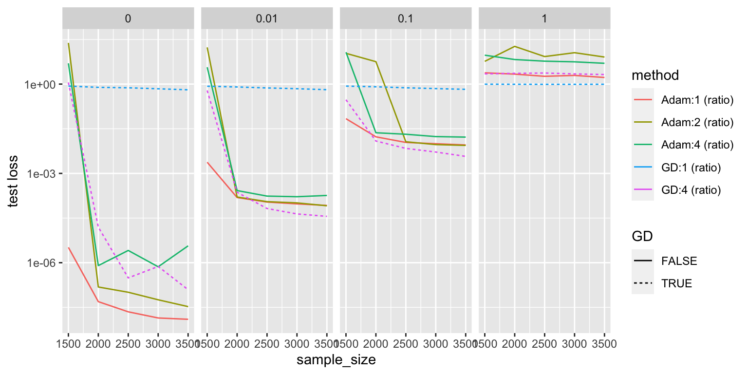
It looks like depth 1 Adam is the king!