#neural_networks
Transformers
- references:
- lil-log
- distill
- ebook-chapter on transformers (actually this ebook isn’t great, as it ends up being more about the implementation)
- it turns out that #attention is an earlier concept, which itself is motivated by the encoder-decoder sequence-to-sequence architecture
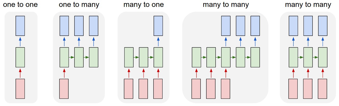
- (oops) I didn’t really understand this diagram:
- sequence to sequence models are essentially the third diagram, where basically the input sequence and output sequence are asynchronous
- versus the normal rnn, which takes the output as the input
- I really like the example of 1-to-many, image-to-caption, so your input is not a sequence, but your output is
- seq2seq example is the translation program, where importantly the input and output sequence don’t have to be the same length (due to the way languages differ in their realizations of the same meaning)
- the encoder is the rnn on the input sequence, and this culminates into the last hidden layer
- this is essentially the context vector: the idea here is that this (fixed-length) vector captures all the information about the sentence
- key: this acts like a sort of informational bottleneck, and actually is the impetus for the attention mechanic
- this is essentially the context vector: the idea here is that this (fixed-length) vector captures all the information about the sentence
- key point (via this tutorial):
- instead of having everything represented as the last hidden layer (fixed-length), why not just look at all the hidden layers (vectors representing each word)
- but, that would be variable length, so instead just look at a linear combination of those hidden layers. this linear combination is learned, and is basically attention
- Transformers #todo
- “prior art”
- CNN: easy to parallelize, but aren’t recurrent (can’t capture sequential dependency)
- RNN: reverse
- goal of transformers/attention is achieve parallelization and recurrence
- by appealing to “attention” to get the recurrence (?)
- “prior art”
Transformers
- key is multi-head self-attention
- encoded representation of input: key-value pairs (\(K,V \in \mathbb{R}^{n}\))
- corresponding to hidden states
- previous output is compressed into query \(Q \in \mathbb{R}^{m}\).
- output of the transformer is a weighted sum of the values (\(V\)).
- encoded representation of input: key-value pairs (\(K,V \in \mathbb{R}^{n}\))
Todo
- [[toread]]: Visualizing and Measuring the Geometry of BERT arXiv
- random blog
- pretty intuitive description of transformers on tumblr, via the LessWrong community
Backlinks
- [[gpt3]]
- This is a 175b-parameter language model (117x larger than GPT-2). It doesn’t use SOTA architecture (the architecture is from 2018: 96 transfomer layers with 96 attention heads (see [[transformers]])1 The self-attention somehow encodes the relative position of the words (using some trigonometric functions?).), is trained on a few different text corpora, including CommonCrawl (i.e. random internet html text dump), wikipedia, and books,2 The way they determine the pertinence/weight of a source is by upvotes on Reddit. Not sure how I feel about that. and follows the principle of language modelling (unidirectional prediction of next text token).3 So, not bi-directional as is the case for the likes of #BERT. A nice way to think of BERT is a denoising auto-encoder: you feed it sentences but hide some fraction of the words, †and BERT has to guess those words. And yet, it’s able to be surprisingly general purpose and is able to perform surprisingly well on a wide range of tasks (examples curated below).
Discretization of Gradient Flow
Via [[michael-jordan-plenary-talk]], to this paper on arXiv.
You have gradient descent, which you can show under convex problems to have a convergence rate of \(\frac{1}{t}\), whereas if you use Nesterov’s accelerated gradient method gets \(\frac{1}{t^2}\).1 And this rate is entirely independent of the ambient dimension of the space.
If you take the limit of the step sizes to zero, then you’re going to get some kind of differential equation. This is gradient flow. It turns out you can basically construct a class of Bregman Lagrangians, which essentially encapsulate all the gradient methods.
You can solve the Lagrangians for a particular rate, and then out pops an differential equation that obtains that rate in continuous time. What’s curious is that the path is identical across all these ODEs. Essentially you’re getting path-independence from the rate, which suggests that this method has found an optimal path, and you can essentially tweak how fast you want to go along that path.
This would suggest that you could then get arbritrary rates for your gradient method. But it turns out that the discretization step is where things break. In fact, Nesterov already has a lower bound on his rate of \(\frac{1}{t^2}\),2 The class of gradient methods are those that have access to all past gradients, I think. so we know it can’t do arbitrarily well. And it turns out that it does match the lower bound. The intuition is that the discretization suffers with curvature. If you go too quickly, then you’re not going to be able to read the curvature well enough.
In other words, discretization is non-trivially different to continuous time. Which sort of makes sense, since in continuous time you have basically all the information.
Finally, in relation to the [[project-penalty]], this doesn’t actually work for things like Adam, which we know to be amazing in practice. So, it seems like there’s still work left to understand why on earth the adaptive learning rates work so well.
Backlinks
Graph Network as Arbitrary Inductive Bias
src.
The architecture of a neural network imposes some kind of structure that lends itself to particular types of problem (CNN, RNN). Thus, you can think of this as some form of inductive bias. An interesting view of [[graph-neural-networks]] is that essentially these provide arbitrary inductive bias, since the goal is to learn the architecture?
| Component | Entities | Relations | Inductive Bias | Invariance |
|---|---|---|---|---|
| FC | Units | All-to-all | Weak | - |
| Conv. | Grid elements | Local | Locality | Spatial transl. |
| Recurrent | Time | Sequential | Sequentially | Time transl. |
| Graph | Nodes | Edges | Arbitrary | V,E permute |
From (Battaglia et al. 2018Battaglia, Peter W, Jessica B Hamrick, Victor Bapst, Alvaro Sanchez-Gonzalez, Vinicius Zambaldi, Mateusz Malinowski, Andrea Tacchetti, et al. 2018. “Relational inductive biases, deep learning, and graph networks.” arXiv.org, June. http://arxiv.org/abs/1806.01261v3.)
(Though, is that really what GNNs really do?)
Network Pruning
(Blalock et al. 2020Blalock, Davis, Jose Javier Gonzalez Ortiz, Jonathan Frankle, and John Guttag. 2020. “What is the State of Neural Network Pruning?” arXiv.org, March. http://arxiv.org/abs/2003.03033v1.): NN pruning is an iterative method whereby you train a network (or start with a pre-trained model), prune based on assigned scores to structures/parameters, then retrained (since the pruning step will usually reduce accuracy), which is known as fine-tuning.
Backlinks
- [[problems-with-machine-learning-scholarship]]
- Pruning: [[network-pruning]]
The Form of the Loss in Matrix Completion
Key: everything goes through the loss function!
What’s wacky is that, usually when we think of neural networks, we have some data pairs \((x,y)\), and the usual operation is that you feed your input \(x\) into your network, and out pops your prediction of \(y\). Another way to put that is, you assume that \(y = f(x)\) for some unknown function \(f\), and the goal of training a neural network is to emulate that unknown \(f\).
In particular, if you ignore the non-linear components, and we deal with a fully connected neural network, then what it boils down to is repeatedly hitting the input vector \(x\) with weight matrices \(W_1, W_2, \ldots, W_N\).
Everything gets turned on its head, it feels, when you consider the problem of Matrix Completion. The architecture is exactly the same, except now the \(x\)’s have disappeared, and what you’re left with are just the weight matrices, and the way you use them is all through this new loss function:
\[ \begin{align*} \norm{ P_{\Omega}(\hat{W}) - P_{\Omega}(W) }_{2}^2, \end{align*} \]
where the \(P_{\Omega}\) is the vectorized form of the relevant entries shown in \(W\), and the \(\hat{W}\) is precisely the product of all the individual weight matrices (since it’s linear it’s equivalent to hitting \(x\) with one matrix). Thus, there’s not really a nice one-to-one in terms of what \((x,y)\) are here. But those are ultimately superfluous.
Really, everything can be derived through the loss function. That is, the normal loss function looks like:
\[ \begin{align*} \sum_{i} L(y_i, f(x_i)). \end{align*} \]
The diagrams we build to describe our networks can sometimes be misleading.
Backlinks
- [[extending-the-penalty]]
- currently, in the case of matrix completion, the penalty is straightforward, since we have a product matrix already as our final goal [[the-form-of-the-loss-in-matrix-completion]].
A Snide Comment about Certain Types of Research
While cleaning out my Dropbox account, I stumbled upon a collection of papers I had saved, almost a decade back. While browsing one of them (The Pulse of News in Social Media: Forecasting Popularity: arXiv), I couldn’t help notice parallels with the current papers I’m reading regarding [[project-misinformation]].
What’s funny is that back in 2012, the state of the art was well summarized by Figure 1. And this aligned almost exactly with what we were taught in our ML class. And now, of course, every paper is basically using neural networks, which again matches the state of the art.
 Figure 1: State of the Art in 2012!
I mean, at some level, this is just a comment about how ideas get circulated. Statistics and ML proffer methodologies that can then be applied to different problems to gain insight. It’s the natural sequence of events in science. At some other level, it sort of shows how derivative a lot of research really is. Of course, someone needs to apply the methods. And I guess people should be compensated for doing the labor (in the form of a publication).
I do think that something has changed in recent years. The flexibility of neural networks, and the need to play with the architecture, means that you can do cutting-edge research simply by trial and error. It has definitely moved more into the real of engineering. Another way to think about this is that, we used to worry about feature engineering, which is that you would spend a lot of time trying to create the right covariates to them input into your standard classification method. Now, we simply do feature-extraction engineering.