Linear Networks via GD Trajectory

Setup

In a linear network, we have \(N\) matrices (weight matrices, parameters), the product of which \(W_N \ldots W_1 = W_{1:N}\) we call the end-to-end matrix. This is what we use in the loss function.

Note that when we actually calculate the gradient, we’re going to be doing it for all the individual matrices/parameters. But it turns out that there’s an equivalence between this natural gradient flow (what actually gets implemented), and the one if you were to consider the single-layer version.

Figure 1: Comparison between the two equivalent linear models

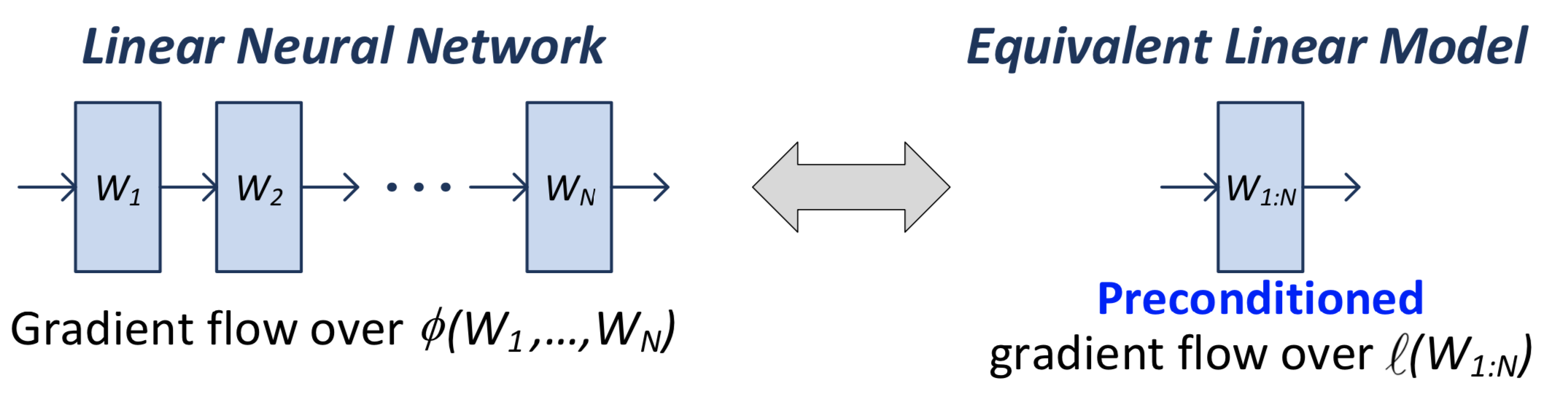
What you can show is that the gradient flow of the \(W_{1:N}\) matrix is equivalent to a pre-conditioned version of the single-layer gradient:

\[ \begin{equation} \frac{d}{dt} \operatorname{vec}\left[ W_{1:N}(t) \right] = - P_{W_{1:N}(t)} \cdot \operatorname{vec}\left[ \nabla l( W_{1:N}(t)) \right] \tag{1} \end{equation} \]

Thus, adding additional (redundant) linear layers induces “preconditioners promoting movement in directions already taken”.[^ Preconditioners are linear transformations that condition a problem to make it more suitable for numerical solutions, and usually involve reducing the condition number. It turns out that the ideal preconditioner is the M-P pseudo-inverse, which we’ve seen before, [[pseudo-inverses-and-sgd]].]

Recall that the condition number is the ratio of the max to the min singular value, so relates to how much the matrix scales the input.

Important: this above analysis (1) is independent of the form of the loss function. I think the only requirement is that the parameters come into the loss function through the end-to-end matrix.

Equivalent Explicit Form?

So, we see that depth plays this role of preconditioning. A question is, does there exist some other loss function \(F\) such that

\[ \begin{equation*} \frac{d}{dt} \operatorname{vec}\left[ W_{1:N}(t) \right] = - P_{W_{1:N}(t)} \cdot \operatorname{vec}\left[ \nabla l( W_{1:N}(t)) \right] = - \operatorname{vec}\left[ \nabla F (W_{1:N}(t)) \right]. \end{equation*} \]

That is, is there just some particularly smart loss function that you could pick that is able to recreate this depth effect? It turns out the answer is no. At this point, we should be talking about the particular matrix completion loss function. The proof involves: by the gradient theorem, we have that, for some closed loop \(\Gamma\),

\[ \begin{align*} 0 = \int_{\Gamma} \operatorname{vec}\left[ \nabla F (W) \right] dW = \int_{\Gamma} P_{W} \cdot \operatorname{vec}\left[ \nabla l(W) \right] dW. \end{align*} \]

Turns out you need some technical details, involving actually constructing a closed loop, the details of which can be found on page 6 of (Arora, Cohen, and Hazan ⊕2018Arora, Sanjeev, Nadav Cohen, and Elad Hazan. 2018. “On the optimization of deep networks: Implicit acceleration by overparameterization.” In 35th International Conference on Machine Learning, Icml 2018, 372–89. Institute for Advanced Studies, Princeton, United States.).

Ultimately, this is not particularly interesting, because a) it’s an exact statement: okay, there’s no explicit choice of loss function that exactly replicates this, but that doesn’t prevent there from being something arbitrarily close; and b) …11 So actually I was going to say that, this is a strawman argument, since they are dealing with an essentially degenerate linear network so clearly you can’t do any better than something like convex programs (and it’s just barely even overparameterized?). But now I’m realizing that we never did depth 1, since it just felt silly. But perhaps depth 1 actually works too. Time to find out…

Optimization

Consider again (1). Murky on the details (see slides), but since \(P_{W:N}(t) \succ 0\), then the loss decreases until \(\nabla l(W_{1:N}(t)) = 0\). Then under certain conditions (\(l\) being convex), this means gradient flow converges to a global minimum.

What this is saying: for arbitrary convex loss function, running a DLNN gives a global minimum. If loss is \(l_2\), you can actually get a linear rate of convergence.

This stuff is pretty cool, simply because gradient descent really shouldn’t have any global guarantees. The only way for you to be able to have global guarantees is if you have some control over the trajectory.

Note though that this doesn’t say anything about generalization performance.