Testing a PA model

Testing Problem

We are interested in the following testing problem: how do we distinguish between a graph generated from a PA model, and a graph from a configuration model with the same degree distribution as the first graph?

The point of this test is, in part, to determine what are the defining properties of a PA model besides the fact that it is scale-free. Of course, we consider the undirected version, as otherwise it would be trivial (since PA vertices all have an out-degree of \(m\)).

Our first idea was to take inspiration from (⊕Bubeck, Devroye, and Lugosi 2014Bubeck, Sébastien, Luc Devroye, and Gábor Lugosi. 2014. “Finding Adam in random growing trees.” arXiv.org, November. http://arxiv.org/abs/1411.3317v1.), and consider centroids11 defined as the vertex whose removal results in the minimum largest component. However, given the lack of an off-the-shelf implementation of this algorithm in R, we decided to look for a simpler test. As it turns out, if we just look at the nodes with the highest degree (together), we get interesting results.

set.seed(5)
library(igraph)
# create induced subgraph by taking the k largest degree nodes
create_induced_topk <- function(g, k) {
  n <- gorder(g)
  dg <- degree(g)
  induced_subgraph(g, order(dg)[(n-k+1):n])
}
# compares to graphs g,h to test which is which
tester <- function(g, h, k=20) {
  g2 <- create_induced_topk(g, k)
  h2 <- create_induced_topk(h, k)
  # if sizes are the same, we should return 1/2
  ifelse(gsize(g2) == gsize(h2), .5, gsize(g2) < gsize(h2))
}

Consider the following test: for a graph \(G\), calculate the induced subgraph by taking the top-\(k\) degree vertices. Which model produces an induced subgraph with more edges?

n <- 100
k <- 5
g <- sample_pa(n, power=1, m=2)
(g2 <- create_induced_topk(g, k))

## IGRAPH 99eb979 D--- 5 7 -- Barabasi graph
## + attr: name (g/c), power (g/n), m (g/n), zero.appeal (g/n), algorithm
## | (g/c)
## + edges from 99eb979:
## [1] 2->1 3->1 3->2 4->1 4->3 5->1 5->4

h <- sample_degseq(degree(g), method="vl")
(h2 <- create_induced_topk(h, k))

## IGRAPH bdfa659 U--- 5 6 -- Degree sequence random graph
## + attr: name (g/c), method (g/c)
## + edges from bdfa659:
## [1] 1--2 3--4 1--5 2--5 3--5 4--5

par(mfrow=c(1,2))
Plot(g2)
Plot(h2)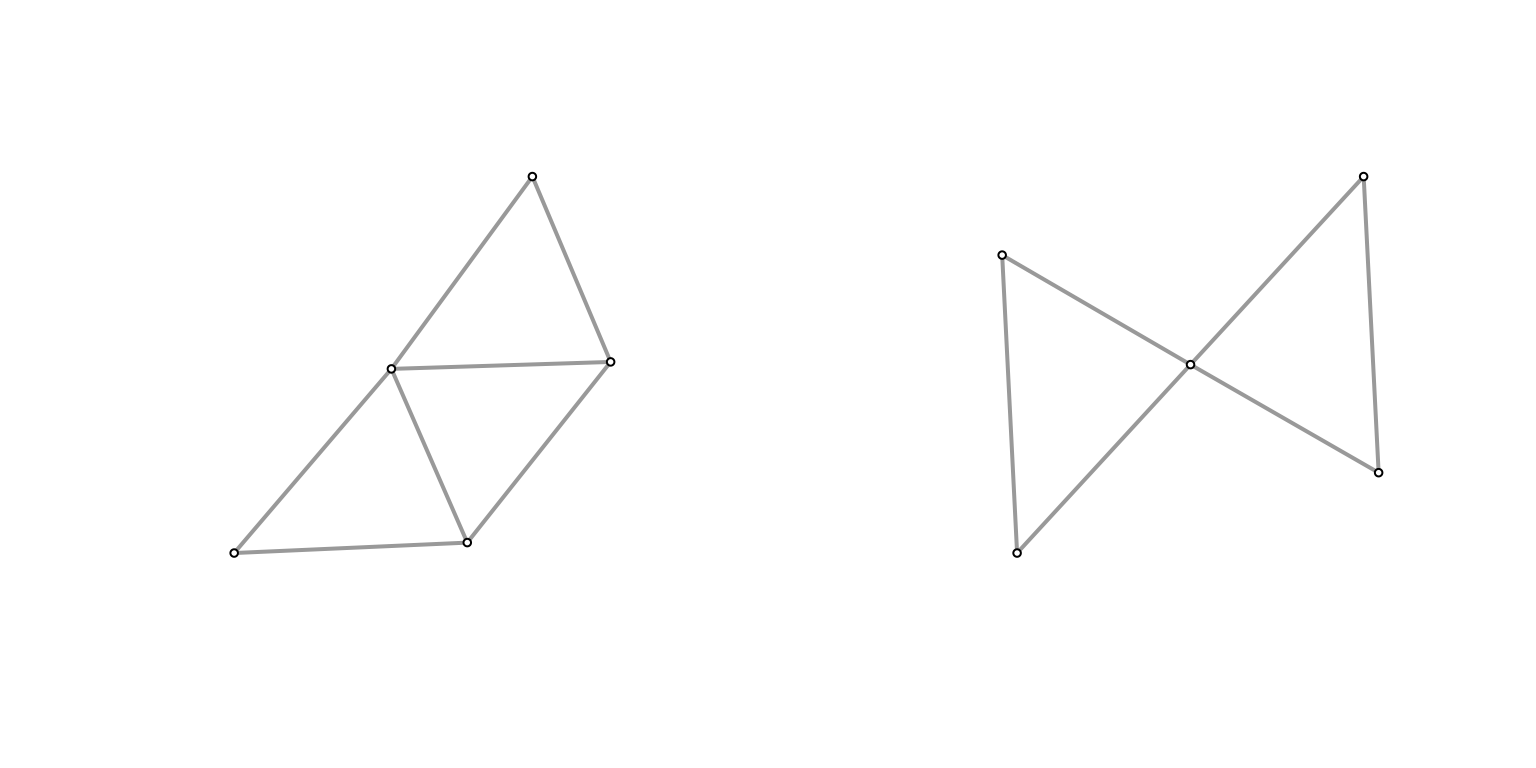

They don’t look that different at \((n,k) = (100,5)\), and the size of the graph is similar (edge count). What if we turn it up a notch?

n <- 1000
k <- 10
g <- sample_pa(n, power=1, m=2)
(g2 <- create_induced_topk(g, k))

## IGRAPH fdeb1f2 D--- 10 13 -- Barabasi graph
## + attr: name (g/c), power (g/n), m (g/n), zero.appeal (g/n), algorithm
## | (g/c)
## + edges from fdeb1f2:
##  [1]  2->1  3->1  3->2  4->1  4->3  5->1  6->2  7->4  7->6  8->1  9->3  9->6
## [13] 10->3

h <- sample_degseq(degree(g), method="vl")
(h2 <- create_induced_topk(h, k))

## IGRAPH 1468645 U--- 10 22 -- Degree sequence random graph
## + attr: name (g/c), method (g/c)
## + edges from 1468645:
##  [1] 1-- 3 2-- 3 1-- 4 2-- 4 3-- 4 1-- 5 2-- 5 1-- 6 2-- 6 4-- 6 3-- 7 4-- 7
## [13] 1-- 8 3-- 8 6-- 8 7-- 8 1-- 9 3-- 9 1--10 3--10 4--10 5--10

par(mfrow=c(1,2))
Plot(g2)
Plot(h2)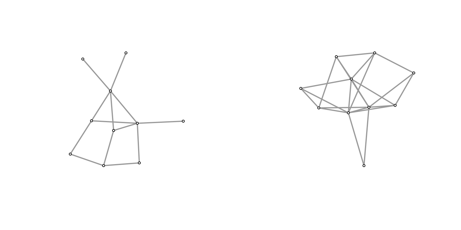

It feels like the induced subgraph from the configuration model is more densely connected (closer to a clique). Why might this be? In the case of the configuration model, if you consider the top \(k\) degree’d vertices, then there’s a very high probability of them being connected to one another22 if we take the half-edge formulation, then for any half-edge, it’s more likely to be connected to those with higher degrees (since they possess more half-edges). but they themselves have more half-edges, so it should amount to more edges between them.. Meanwhile, for a PA model, roughly we have that high degree nodes are older/earlier, and so probably have a slightly larger chance of connecting to each other than, say, a younger and an older node (since early on there aren’t many other options), but this is probably a much smaller effect.

To test this, let’s run some simulations. Here, I’ve run all combinations of \(n \in [100, 500, 1000]\) and \(k \in [5, 10, 15]\).

nsim <- 1000
ns <- c(100, 500, 1000)
ks <- c(5, 10, 20)
df <- expand.grid(k=ks, n=ns)
df$prob <- 0
cnt <- 1
for (k in ks) {
  for (n in ns) {
    res <- c()
    for (i in 1:nsim) {
      # generate graph
      g <- sample_pa(n, power=1, m=2)
      # generate the equivalent configuration model
      h <- sample_degseq(degree(g), method="vl")
      res <- c(res, tester(g, h, k=k))
    }
    df$prob[cnt] <- mean(res)
    cnt <- cnt + 1
  }
}
knitr::kable(df)

k	n	prob
5	100	0.7475
10	100	0.8180
20	100	0.8705
5	500	0.9740
10	500	0.9940
20	500	0.9980
5	1000	0.9990
10	1000	1.0000
20	1000	1.0000

Clearly, we see a positive relationship between both \(k\) and \(n\) with respect to testing accuracy. Though, at \(n=1000\), it’s essentially as good as it’s going to get.

“Theory”

Here’s some hand-wavy calculations. For the simplest case of \(k=2\), we are interested in the probability that the top two degree vertices are connected. Let \(d_1, d_2\) be these degrees (and the respective vertex too). For the configuration model, for any given half-edge of \(d_1\), the probability that it’ll be connected to \(d_2\) is given by \(\dfrac{d_2}{D - d_1}\). Then, the probability that they’re connected is given, roughly, by \(\dfrac{d_1 \cdot d_2}{D}\).

Now consider the preferential attachment model. For now, let’s assume that \(d_1\) arrived before \(d_2\).33 can’t really WLOG here, but it feels close enough In other words, what we’re interested is the probability that one of the \(m\) vertices chosen by \(d_2\) was \(d_1\). Denote the arrival time44 which also corresponds to the number of vertices at that time of these two vertices as \(t_1\) and \(t_2\), respectively. Then, the probability is given by \(\dfrac{d_1(t_2)}{m \cdot t_2}\). The further out the \(t_2\), the larger the denominator, but also the more time \(d_1\) has had to amass its popularity.

The key is that it’s independent of \(d_2\) (i.e. the degree of the second vertex) – it would be the same probability for any other node at time \(t_2\).