Matrix Completion Optimization
tags: [ lit_review , proj:penalty , matrix_completion , optimization ]
Let’s try to understand the landscape of optimization in matrix completion.
Matrix Factorization
A celebrated result in this area is (Ge, Lee, and Ma 2016Ge, Rong, Jason D Lee, and Tengyu Ma. 2016. “Matrix completion has no spurious local minimum.” In Advances in Neural Information Processing Systems, 2981–9. University of Southern California, Los Angeles, United States.). They consider the matrix factorization problem (with symmetric matrix, so that it can be written as \(XX^\top\)). Note that this problem is non-convex.1 The general version of this problem, with \(UV^\top\), interestingly, is at least alternatingly (marginally) convex (which is why people do alternating minimization). Under some typical incoherence conditions,2 To ensure that there is enough signal in the matrix, preventing cases where all the entries are zero, say. they are able to show that this optimization problem has no spurious local minima. In other words, for every optima to the function \[ \begin{align*} \widetilde{g}(x) = \norm{ P_\Omega (M - X X^\top) }_F^2, \end{align*} \] it is also a global minima (which means \(=0\)).3 They were inspired, in part, by the empirical observation that random initialization sufficed, even though all the theory required either conditions on the initialization, or some more elaborate procedure.
Proof technique: they compare this sample version \(\widetilde{g}(x)\) to the population version \(g(x) = \norm{ M - X X^\top }_F^2\), and use statistics and concentration equalities to get desired bounds.
Remark. The headline (no spurious minima) sounds amazing, but it’s not actually that non-convex. In any case, as it turns out, it’s basically non-convex (i.e. multiple optima) because you have identifiability issues with orthogonal rotations of the matrix (that cancel in the square). I wonder if the incoherence condition is important here. I don’t think so, as it’s a pretty broad set, so it really does seem like this problem is pretty well-behaved.
A nice thing about the factorization is that zero error basically means you’re done (given some conditions on sample size), since having something that factorizes and gets zero error must be the low-rank answer.To reiterate, they don’t use any explicit penalty (except something that’s helpful for the proof technique to ensure you are within the coherent regime). The matrix factorization form suffices.
Important: something I missed the first time round, but actually makes this somewhat less impressive: they basically assume the rank is given, and then force the matrix to have that dimension. This differs from (Arora et al. 2019Arora, Sanjeev, Nadav Cohen, Wei Hu, and Yuping Luo. 2019. “Implicit Regularization in Deep Matrix Factorization.” arXiv.org, May. http://arxiv.org/abs/1905.13655v3.)’s deep matrix factorization as there they aren’t forcing the dimensions. This doesn’t seem that impressive anymore.
Non-Convex Optimization
src: off-convex.
The general non-convex optimization is an NP-hard problem, to find the global optima. But even ignoring the problem of local vs global, it’s even difficult to differentiate between optima and saddle points.
Saddle points are those where the gradients in the direction of the axis happen to be zero (usually one is max, the other is a min). In the case of gradient descent, since we move in the direction of gradient for each coordinate separately, then we’re basically stuck.
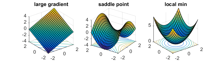
If one has access to second-order information (i.e. the Hessian), then it is easy to distinguish minima from saddle points (the Hessian is PSD for minima). However, it is usually too expensive to calculate the Hessian.
What you might hope is that the saddle points in the problem are somewhat well-behaved: there exists (at least) one direction such that the gradient is pretty steep. This way, if you can perturb your gradient, then hopefully you’ll accidentally end up in that direction that lets you escape it.
That’s where noisy gradient descent (NGD) comes into play. This is actually a little different to stochastic gradient descent, which is noisy, but that noise is a function of the data. What we want is actually to perturb the gradient itself, so you just add a noise vector with mean 0. This allows the algorithm to effectively explore all directions.4 In subsequent work, it has been established that gradient descent can still escape saddle points, but asymptotically, and take exponential time. On the other hand, NGD can solve it in polynomial time.
What they show is that NGD is able to escape those saddle points, as they eventually find that escape direction. However, the addition of the noise might have problems with actual minima, since it might perturb the updates sufficiently to push it out of the minima. Thankfully, they show that this isn’t the case. Intuitively, this feels like it shouldn’t be that hard – if you imagine a marble on these surfaces, then it feels like it should be pretty easy to perturb oneself to escape the saddles, while it seems fairly difficult to get out of those wells.
Proof technique: replace \(f\) by its second-order taylor expansion \(\hat{f}\) around \(x\), allowing you to work with the Hessian directly. Show that function value drops with NGD, and then show that things don’t change if you go back to \(f\). In order for this to hold, you need the Hessian to be sufficiently smooth; known as the Lipschitz Hessian condition.
It turns out that it is relatively straightforward to extend this to a constrained optimization problem (since you can just write the Lagrangian form which becomes unconstrained). Then you need to consider the tangent and normal space of this constrain set. The algorithm is basically projected noisy gradient descent (simply project onto the constraint set after each gradient update).